

Understanding LLM Inference
Explaining LLM pre-fill and generation phases, unpacking model configuration files from HuggingFace.

In this article, you’ll learn about:
Model Inference and Serving
How next tokens are sampled
LLM Model Files on HuggingFace
Parameters and LLM Configurations
A majority of recent advancements in AI research have been driven by scale.
In 2023, Ilya Sutskever, OpenAI Co-Founder, said this in an interview:
I. Sutskever
Ilya’s quote holds value as scale remains the underlying factor that new SOTA models follow today. In 2020, AI research scientists published the “Scaling Laws for Neural Language Models” [7] research paper where they studied the empirical scaling laws for language models performance as a result driven by 3 factors:
Compute
Dataset Size
Parameters Count

In short, the most notable observation was that LLM performance improves smoothly as we increase the model size, dataset size, and computing used for training. That also affects the inference process, as bigger models require more computing to be served efficiently and within reasonable latency boundaries.
In this article, we’ll see exactly how Inference works in LLMs. Using a custom prompt as an example, we'll go through the prefill and generation phases step-by-step. While doing that, we’ll explain the workflow of token sampling, Linear Projection, and how Softmax is applied to logits to get probability distributions of the next tokens.
We’ll show how TopN, TopK, and Temperature impact token selection and how the generation stops.
Finally, we’ll unpack each model configuration file that is part of an LLM model on HuggingFace, explaining the architecture config, generation config, model weights partitions, and layer mappings - which will help us understand why LLMs don’t require only weights files, but also quite a few config files to prepare them for fine-tuning or inference.
Table of Contents
What is Model Inference and Serving
Inference in GenAI Models: Types of LLM Models
The Prefill and Decode Inference Stages
[New] How a Decode step flows through the GPU
[New] The 4 Inference Patterns
[New] Challenges with LLM Inference
Unpacking LLM Model Files on Hugging Face
Model Architecture Config
Tokenizer and Special Tokens
Generation Config
Model Weights and Layers Index
Conclusion
What is Model Inference and Serving?
In the MLOps Lifecycle, the inference process is part of the deployment and feedback stage. Once we’ve gathered data, cleaned and prepared it for training, iterated over training experiments, and selected the best model, it’s time to deploy and feed real-world, unseen data to obtain predictions.
By inference, we understand the process of feeding a trained model and unseen input data (inference data) to obtain predictions as output, which are consumed by a user or service.
Furthermore, model serving refers to packaging and deploying a model, making it available as real-time feed processing services or API invokable services in production environments. [2]
In a simplified format, a model is nothing more than a graph of structured mathematical operations organized in layers, with predefined constants as weights & bias values attached to each Neuron or Layer as learned parameters through the model training process. To make a model deployable, we have to set libraries, frameworks, dependencies, and pipelines to process the input data to a standardized format that our model could understand and, vice-versa, to unpack model outputs (i.e., predictions) to a format compatible with our application.
2. Inference in GenAI Models: Types of Models
All LLM models that do completions, such as GPT-4, 4o, Gemini, Claude, Llama, or Mistral, are Decoder-Only models. That’s because they’re trained to predict the next token in a sequence, given all previous tokens.
Hence the name “causal” decoding or “autoregressive” language models.
Most popular decoder-only LLMs are pre-trained on causal modeling as next-word predictors. They take a series of tokens as inputs and continue generating the next token of the sequence until they’ve met a stopping criterion, either a special token such as <end>, <eos>, <end_of_text>, or have reached the specified max_tokens argument.
These special tokens differ depending on the LLM training configuration, such as the Tokenizer and Vocabulary the LLM was trained with.
These models are highly efficient for tasks such as text generation, summarization, and dialogue, as they process information in a left-to-right fashion, without requiring the full input sequence to be seen all at once.
However, they differ from Encoder-Decoder models, which have a fundamentally different architecture and training approach.
Encoder-Decoder models, like T5 or BART, are trained with a sequence-to-sequence objective. Here, the encoder first compresses the input sequence into a latent representation, and then the decoder generates output tokens based on that representation.
The encoder-decoder model is well-suited for translation, where the model needs to fully understand the input sentence in source language before starting to generate an output in target language.
In short:
Decoder Only → open-ended generation and completions.
Encoder-Decoder → requires the full input before generating a response.
Since we’re focusing on Decoder-Only architectures in this article, let’s explain the inference stages: Prefill and Decode.
3. The Prefill and Decode Inference Stages
This inference process is autoregressive, as the T0… T(n-1) tokens generate the T(n) token, and subsequently, T0... T(n) generates the T(n+1) token.
During this process, we must understand the 2 phases involved in LLM inferencing: the prefill (init) phase and the decode (generate) phase.
Before diving into Prefill and Decode in detail, let’s focus a bit on how LLM inputs flow through the GPU to create a better understanding
The LLM Prefill Phase
Prefill is also known as processing the input; this is where the LLM takes tokens as input and computes intermediate states (keys and values), which are used to generate the “first” new token.
Let’s take “Neural Bits Newsletter is” as our input text for an example. During prefill, our text is tokenized, and the model goes through a “warm-up” stage to compute the initial K and V matrices from this input text.
For inference, it is important to note that the prefill phase efficiently saturates the GPU memory because the model sees the entire input context on the first prompt. The attention mechanism at this stage can be considered a matrix-to-matrix operation, which is highly parallelizable on GPUs.
ℹ️ Each LLM model trains it’s own tokenizer, and this is highly tied to the text corpus used as the pre-training dataset. The following example uses the GPT-4o and GPT-4o-mini tokenizer from [6].

A nice metric to count for is TTFT (time to the first token), which measures the prefill time, tokenization, and initial K, V states computation. It is usually used to test the performance of the prefill stage.
Once the first next token was added to the sequence, we entered the autoregressive generation phase.
After this stage, the Q, K, and Attention Matrices states are “warmed up,” and the generation runs faster, as the memory was already allocated.
The LLM Generation Phase
Generation describes the LLM’s autoregressive process of yielding tokens one at a time until a stopping criterion is met. Each sequential output token needs to know all the previously generated tokens' previous output states (keys and values).
One important note here is that the Generation phase is memory-bound. Let’s explain that.
The speed at which the weights, keys, values, and activations are transferred to the GPU from the CPU memory is slower than the actual compute time required to get these in the first place. Each new token, key, and value scales linearly, and attention computation scales roughly quadratically.
To understand this scaling relationship, look at the following image [5], showing how the input prompt embeddings flow through the Transformer layers.

At each network layer, the model computes Query (Q), Key (K), and Value (V) vectors for each token in the input sequence and an attention matrix. These representations are refined and more contextually aware as they pass through deeper layers.
Adding a token to the sequence linearly increases the number of rows in the Q, K, and V matrices. The attention matrix, N x N, where N is the sequence length, grows to include the new token, thus scaling the number of attention calculations quadratically.
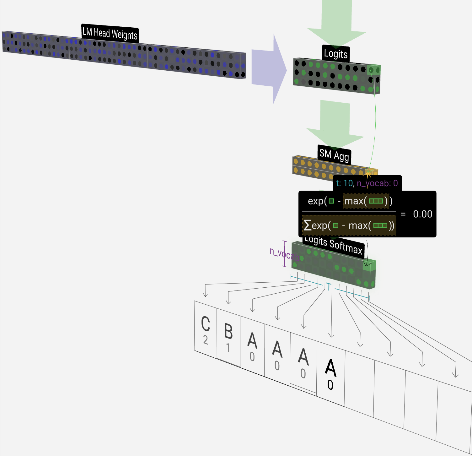
Another fundamental component in LLMs is the last layer, which is, in essence, a classification layer.
This layer involves a Linear Projection (where we map the intermediate outputs from previous layers into n_vocab dimensions, where n_vocab represents the size of the vocabulary the model was trained with.
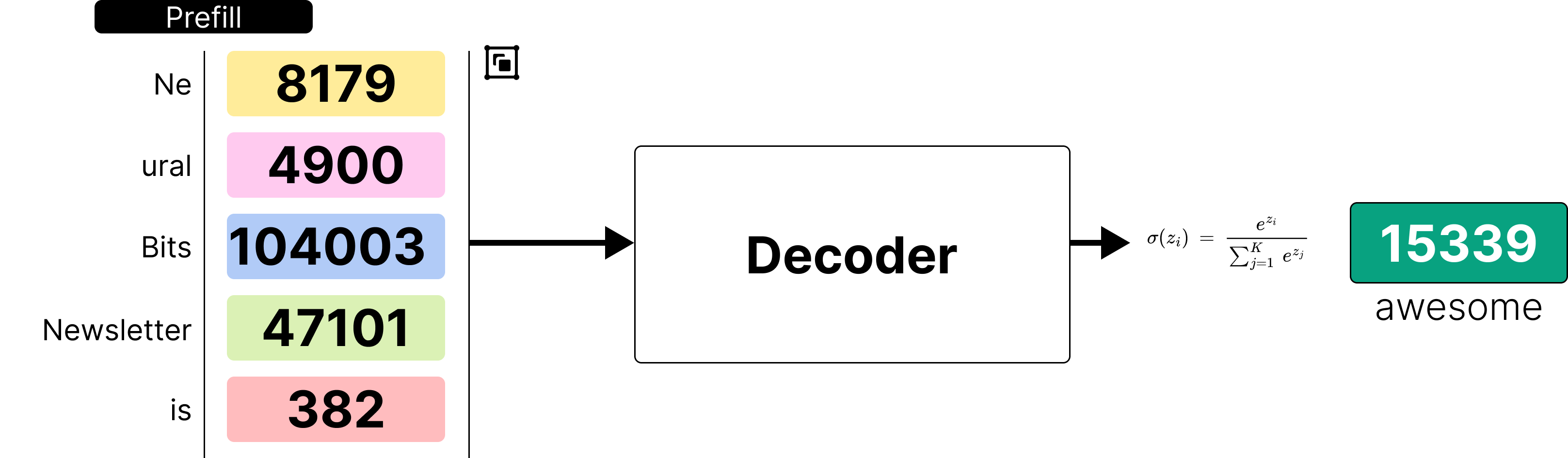
More simply, if our model knows 100 tokens, the logits shape after Linear Projection would be (100). Passing these logits through a Softmax activation gives us a probability distribution over the entire vocabulary, representing the likelihood of each token being the next token. Next, based on the generation config parameters (TopK, TopP, Temperature), the LLM selects the best “next token” and adds it to our sequence, and the process repeats.
We can view this entire process in the following image:
To unpack the generation config arguments mentioned above, we can control the behavior of the token sampling process by modifying the Temperature, TopK, and TopN thresholds. Let’s understand what these arguments do:
Temperature is a scaling factor applied in the final Softmax layer that impacts the probability distribution the model calculates for the next token. A higher Temperature ~= 1 will allow more random/creative token selection, while a lower temperature will lead to more deterministic behavior.
TopK - also known as greedy sampling conditions the model to consider only the K most likely tokens; a lower K will behave deterministic(specifically), while a higher K factor will behave stochastically (randomly).
TopN - also known as nucleus sampling, is similar to TopK. Still, instead of conditioning K tokens to consider, it conditions the cumulative probability of these tokens as the model will select N tokens where the cumulative probability exceeds the threshold.
ℹ️ For example, if we set this to 0.5 and on the first iteration, we have the word “awesome” with a probability of 0.6, it’ll consider this token only. However, if we have “awesome”: 0.1, “amazing”: 0.2, and “marvelous”: 0.3 - it’ll consider all 3 because cummulated, they yield 0.6, which is higher than our threshold.
It's time for a practical example, as it’s much easier to follow.
Let’s go back to our “Neural Bits Newsletter is” prompt above and see what happens after we’ve got our first predicted token “awesome” by following this diagram:

We can quickly observe the repetitive process of appending the new token to the sequence, passing through the model, getting the next token, appending, passing through the model, getting the next token, and so on until we’ve reached the max_tokens limit or the model has predicted a <eos> token that marks the end of the generation.
ℹ️ Now that you’ve learned how that works, whenever you use an LLM model (e.g., ChatGPT, Gemini, Perplexity, or any LLM), that short delay before words start appearing in your chat console is due to prefill and first token generation, and then each new word that appears comes from a generation step.
Awesome! We’ve covered the internals of how LLMs process input and generate new tokens, assuming the model was deployed and ready for us to chat with or send instructions to.
Next, let’s look at a few key metrics to measure the performance of LLM Inference.
4. [New] How a Decode step flows through the GPU
Now that we understand what Prefill and Decode steps are, let’s go one level further and see what happens on the GPU during inference.
Compared to CPUs, GPUs are designed to handle massively parallel computations.
In video games, behind every rendered frame, there is lighting, reflections, object motion, and shadows, all of which are based on math and vector operations. For example, DLSS (Deep Learning Super Sampling) enables a game to render frames at a lower resolution (e.g, 1080p) and then use a deep learning model to upscale it to 4K.
In AI workloads, either training or inference leverages the same types of operations, matrix multiplications, convolutions, normalizations, attention mechanisms, transposes, and other kernels.
During LLM inference:
In the Prefill step, the full input sequence (the prompt) is processed. This involves passing tokens through all the layers of the transformer model, which includes multiple rounds of matrix multiplications, attention, and feedforward operations.
In the Decode step, the model generates one token at a time, reusing the previous computations (KV cache) and processing only the newly generated token through the model.
Both steps are executed on the GPU, where the model’s weights are loaded into high-bandwidth memory (HBM), which is the GPU’s VRAM, and the streaming multiprocessors parallelize the work across.
For more details on GPUs for AI and GPU Programming, read this Starter Guide.
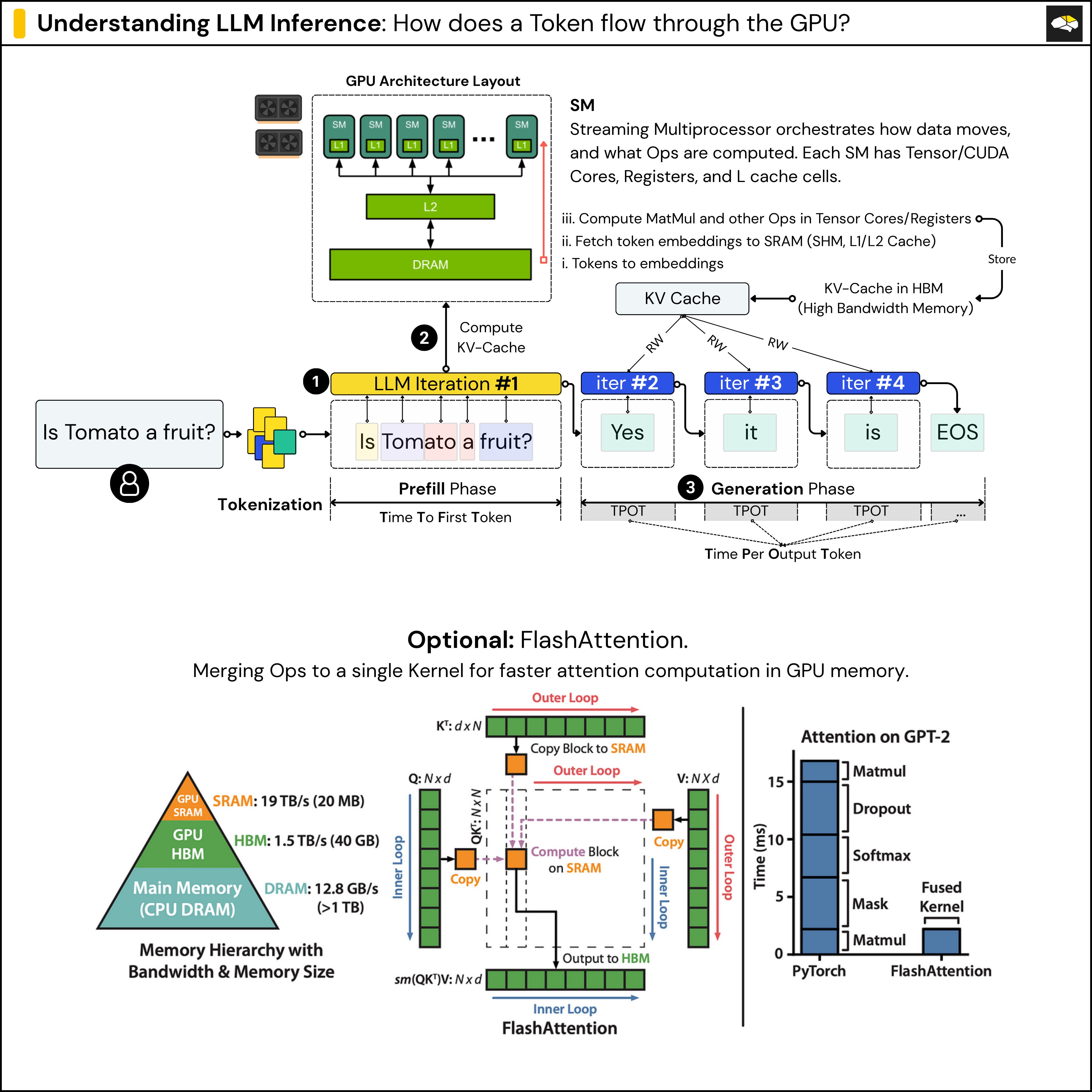
In the image above, after the Tokenization, we pass the tokens through our LLM Model. On the first iteration of inference, each token is converted into an embedding vector.
These embeddings are initially stored in GPU DRAM (also called HBM – High Bandwidth Memory), which has higher latency compared to on-chip memory. To speed up computation, batches of these embedding vectors are loaded into lower-latency memory closer to the compute cores—such as L1/L2 cache or Shared Memory inside the GPU.
This memory slice is local to each Streaming Multiprocessor (SM), and the SM is the unit responsible for executing operations in parallel on the GPU. The SM then moves the data into registers, the fastest type of memory, where actual computations—like attention—are performed using CUDA cores or Tensor Cores.
After computing the attention outputs, the model updates the KV cache (which stores key and value vectors for reuse in later steps). This KV cache is then written back to HBM, making it accessible to the entire GPU for the next token generation steps.
5. [New] Key LLM Inference Metrics
When deploying LLM-based systems to production environments, much like any other Deep Learning model deployment, we have a few important metrics we should keep track of.
Due to how LLM inference works, performance monitoring focuses on the following metrics:
TFTT (Time to First Token) - shows how long a user needs to wait before seeing the model’s output. This is the time it takes from submitting the query to receiving the first token.
TPTO (Time per Token Output) - This is defined as the average time between consecutive tokens, during the generation phase.
RPS (Requests per Second) - This is the average number of requests that can be completed by the system in 1 second.
TPS (Tokens per Second) - This is the average number of tokens the model generates per second, and is a common metric to measure performance.
While these metrics are useful even for models running on a single GPU or a single node with multiple GPUs, they become especially important in large/enterprise-scale deployments.
In these scenarios, models are often sharded across multiple GPUs and nodes, using parallelism techniques such as TP (Tensor Parallel), or PP (Pipeline Parallel).
In such distributed setups, these metrics can help identify performance bottlenecks, such as latency from inter-node communication or inefficient model partitioning across layers.
6. Understanding LLM Model Files from HuggingFace
We talked about how LLM Inference works.
However, we haven’t explained how a model is partitioned and configured. We’ll do that by unpacking a model structure and files that are already a defined standard for sharing LLM weights.
We’ll be using the meta-llama/Meta-Llama-3-8B model from HuggingFace as our example.
To describe HuggingFace shortly, they are the GitHub of open-source AI research.
The discussions and debates on AI research happen on Twitter(X), LinkedIn, and Arxiv with numerous papers.
LLM model repositories, benchmarks, datasets, and leaderboards stay on HuggingFace.
Each model repo on HF usually contains 3 tabs:
The Model Card, where the publishers present the model architecture and report card.
The Files Section, a git-like repository containing the model configuration files and weights. This is the repo that everyone clones to get the model ready to be loaded with HuggingFace’s Transformers library.
The Community Section, similar to Discussion Threads, Issues, or PR’s on GitHub.
We focus on the Files section, as we aim to understand what those are and their usability.
To do that, let’s take a look at the following diagram for Meta-Llama-3-8B:

The highlighted files might differ in namings and structure, but their purpose is the same as they specify:
Model Configuration
The model weights as .bin or .safetensors format
Tokenizer configs, Special tokens, and Layer Mapping
Generation/Inference Config
Let’s unpack them one by one.
Model Configuration
This file contains metadata on model architecture, layer activations and sizes, vocabulary size, number of attention heads, model precision, and more. It can be considered the model core [3], as this file describes the key parameters of our model, which are mandatory to construct and use for fine-tuning or inference.
For this Llama-3-8B example, we can see it was trained in bfloat16 precision on a total vocabulary of 128256 tokens, and it has 32 Attention Heads, 32 Hidden Layers, etc.

Model Weights
Due to LLMs having billions of parameters, the models are usually split into parts for safer download, as no one would like to download an 800GB model and get a network error, ending up with the entire model file being corrupted. These model weights usually come in .bin format as a serialized binary file or .safetensors, a newer format proposed by HuggingFace to safely and efficiently store model files.
Safetensors came mainly as an alternative to the default Pickle serialized that PyTorch was using, as it’s vulnerable to code injection, which is a safety risk. When saving a model as .pt, it uses Pickle underneath, which can serialize Python Objects. One could inject code in a .pt model, and when loading it, Picke will deserialize and execute that code.
Layer Mapping
Since the models are large, and weights come as part files (e.g., 0001-of-0006, 0002-of-0006, etc.), this file stores a sequential map of the model architecture, specifying which part file each layer has its weights.

Tokenizer Config and Special Tokens
The tokenizer config file contains metadata about which tokenizer and configuration were used to train this model. It also shows the class name used to instantiate the tokenizer, the layer names, and how the inputs are processed before passing through the model.
Below is a screenshot of the tokenizer_config.json, where we can see the <bos_token> and <eos_token> this LLM understands and a list of reserved tokens with instructions on how the Tokenizer should process them.

For example, tokenID=128255 is reserved, not a single_word, left_strip and right_strip are false, which means leading and trailing spaces would not be removed using token.strip() method.
In the “special_tokens.json” file, we have the <bos_token> and <eos_token> special tokens mapped to actual text markers that are used in the Chat template or prompt given to this LLM.

As a quick example, the prompt we used above, “Neural Bits Newsletter is” - is not the complete form that gets passed to the Tokenizer. What gets into the tokenizer is this:
<|begin_of_text|>Neural Bits Newsletter isAfter the generation is complete, it’ll become this:
<|begin_of_text|> Neural Bits Newsletter is awesome and helps you learn AI <|end_of_text|>Generation/Inference Config
These configuration files contain metadata for Inference, such as Temperature and TopP/TopK thresholds or context window size the model was trained with. Also, it specifies the tokenIDs for the <bos> and <eos> tokens, such that the Tokenizer can append these ID’s to the sequence.

Conclusion
In this article, we broke down how LLM inference works, covering the Prefill and Generation phases in decoder-only models, which make up a large majority of current LLMs.
These are crucial concepts for understanding both throughput and latency in production deployments of GenAI-based applications.
We then walked through a real prompt example using actual token IDs from the GPT-4o tokenizer, showcasing, step-by-step, how a next token is generated, following the FW layers, Softmax, and Attention computation.
We then examined the structure and purpose of the model files provided on HuggingFace, which is something every AI Engineer should know.
By the end, you not only gained a deeper understanding of how LLMs generate text step by step, but also learned how to navigate and interpret the configuration files that come with these models.
Thank you for reading, see you next week!
References
Hopsworks. (2024). What is Model Serving - Hopsworks. https://www.hopsworks.ai/dictionary/model-serving
meta-llama/Meta-Llama-3-8B at main. (2024, December 6). https://huggingface.co/meta-llama/Meta-Llama-3-8B/tree/main
LLM Visualization. (2025). Bbycroft.net. https://bbycroft.net/llm
OpenAI Platform. (2025). Openai.com. https://platform.openai.com/tokenizer
Kaplan, J., McCandlish, S., Henighan, T., Brown, T. B., Chess, B., Child, R., Gray, S., Radford, A., Wu, J., & Amodei, D. (2020). Scaling Laws for Neural Language Models. ArXiv.org. https://arxiv.org/abs/2001.08361
Topic 23: What is LLM Inference, its challenges, and solutions for it. (2025). Huggingface.co. https://huggingface.co/blog/Kseniase/inference
GPU Performance Background User’s Guide - NVIDIA Docs. (2020). NVIDIA Docs. https://docs.nvidia.com/deeplearning/performance/dl-performance-gpu-background/index.html
Amazing as always ❤️