Building robust ML model pipelines in Triton deployments

Detach processing stages from Python to Triton Inference Server. Build a custom Python Backend and compose a Model Pipeline.

At the end of this article, there’s a poll with 2 options.
Would appreciate your vote, as It’ll help me decide which project to take on next.

In this article, you will learn:

• To build a PythonBackend

• To compose a Model Ensemble in Triton

• About advanced YOLO architecture concepts

---

Deploying ML models to production is not easy work, especially when aiming to strike an optimal balance between performance and quality.

By default, when deploying a model - everyone relies on either:

1. All Inference logic in Python

   1. Which might be slow and non-optimal.

2. Only Pre/Post processing in Python

   1. Model feedforward is handled via a serving framework such as Triton.

In this example, we’ll go with the second option, but in a more advanced and optimized fashion, because we’ll separate the data preparation and model inference stages.

We will use YOLO 11 as our example.

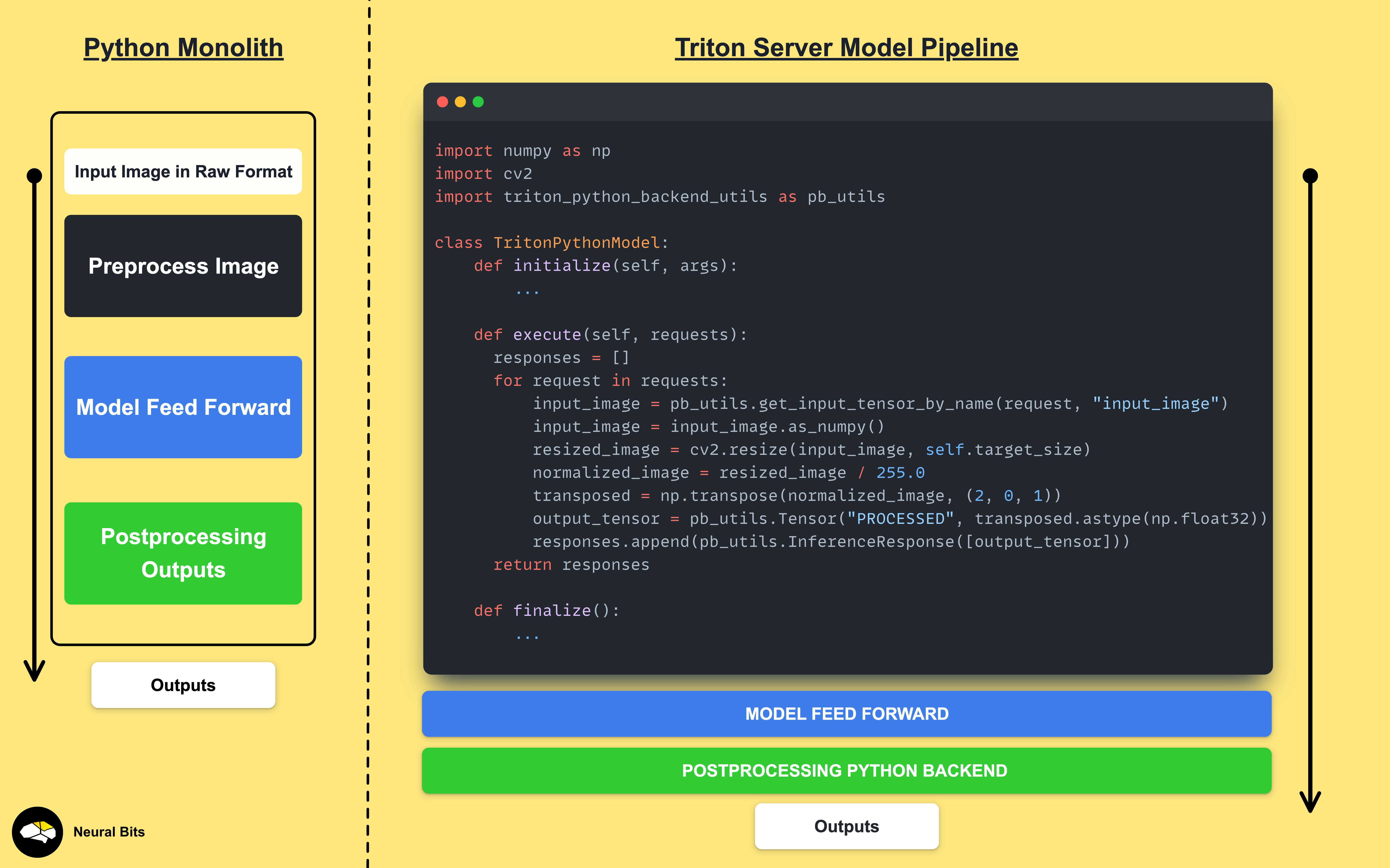
Table of Contents

1. Prerequisites

2. The Plan

3. Stage 1 : Image Preprocessing

4. Stage 2: Model FeedForward

5. Stage 3: Logits PostProcessing

6. Assembling Everything

7. Takeaways

---

Prerequisites

To deploy YOLO 11 efficiently for it to work, it requires these 3 stages:

1. Image Preprocessing

   1. Resizing, color processing, and normalization

2. Model Input FeedForward

3. Logits post-processing

   1. Unpacking the raw output tensor

   2. Cleaning and removing redundant entries

   3. Extracting predictions

Commonly in applications, we will see 1 and 3 handled in Python, and 2, being the most resource-consuming part, done via a ModelServing framework
(e.g ONNXRuntime, TorchScript, Triton/TensorRT, CoreML).

---

The Plan

We will keep Image Preprocessing in Python, Model FeedForward as a compiled and optimized TensorRT Engine, and Logits Postprocessing as a custom Python stage attached to our model.

That way, when we submit an Image Tensor for inference, we’ll get the final outputs, with all the heavy loading being done inside the NVIDIA Triton Server context.

Stage 1: Image Preprocessing

At this stage, we need to resize the image to the expected Model input size and then normalize values in the (0,1) range. Further, we’ll have to re-organize the tensor shape to (N, C, W, H), where:

• N - batch dimension will specify how many images are packed together in a single tensor.

• C - represents the number of channels for color pixels. Color images (RGB) will have a C=3 as each pixel has a RED, GREEN, and BLUE value - whereas a Grayscale image will have C=1.

• W, H - represents the width and height of the Image tensor after the actual image was resized.

# Step 1 - Correct Color
img = cv2.cvtColor(input_image, cv2.COLOR_BGR2RGB)

# Step 2 - Resize to expected size
img = cv2.resize(img, (target_w, target_h), cv2.INTER_LINEAR)

# Step 3 - Normalize
img = np.array(img) / 255.0

# Step 4 - Re-order channels (C, W, H)
img = np.transpose(img, (2, 0, 1))

# Step 5 - Add batch dimension (N)
img = np.expand_dims(img, axis=0)
img = img.astype(target_dtype)

Stage 2: Model Feed Forward

This stage implies that we took the YOLO11 model, compiled it into a TensorRT engine on a specific GPU, and ran a quick test to verify if the Model Graph was correctly generated.

TensorRT engines are the optimal model formats for running inference on NVIDIA GPUs. A TensorRT engine is tightly coupled with the GPU it was compiled on, because the Model Graph structure configures it’s operation kernels depending on the number of CUDA cores, SHM regions and bandwidth.

The workflow of YOLO11 TensorRT compilation is described, with code and detailed steps in this previous article.

---

Stage 3: Logits Postprocessing

The output from the YOLO11 model is a Tensor of the following shape:

(N, n_classes + 4coords * 1score, 8400)

To unpack it, let’s understand how YOLO works under the hood.

YOLO models operate at different scales to handle objects of varying sizes, as the model architecture contains 3 different heads for different object sizes depending on the input image size.

For our example of a 640x640 pixels image, we have:

• Low resolution = grid of 20x20 pixels

• Medium resolution = grid of 40x40 pixels

• High resolution = grid of 80x80 pixels

Credits to RangeKing on Github

For the number of classes, since our YOLO11 model was trained on the COCO dataset, it uses the 80 COCO classes list.

For each grid cell, the model predicts 84 features:

• 4 bounding box coordinates (x,y,w,h)

• 1 objectness score.

• 80 class probabilities (one for each class in the dataset).

Having the grid sizes (20x20, 40x40, 80x80) and the n_classes (80) we get the final shape of:

(N, n_classes + 4coordinates, (20x20 + 40x40 + 80x80)) = (N, 84, 8400)

Since for each grid cell we have a bounding box detection, in the post-processing phase, we need to eliminate duplicates. For that, we’ll wrap the NMS (Non-Maximum-Suppression) algorithm that is applied to the outputs as a custom Python model in our PythonBackend for Triton.

Get the model.py containing our Python Model, and also copy the tools.py script which contains utilities used by our model.

Now, we have to define the actual model to be compatible with the Triton Server. For that, we’ll have to place them under this structure:

model_repository/
└── yolov11-nms/
    ├── 1/
        ├── model.py
    ├── config.pbtxt
    └── tools.py

The config.pbtxt will look like this:

name: "yolov11-nms"
default_model_filename: "model.py"
platform: "python"
max_batch_size: 4

input [
    {
        name: "output0"
        data_type: TYPE_FP16
        dims: [84, 8400]
    }
]

output [
    {
        name: "boxes"
        data_type: TYPE_FP32
        dims: [-1, 4]
    },
    {
        name: "classes"
        data_type: TYPE_INT32
        dims: [-1]
    },
    {
        name: "scores"
        data_type: TYPE_FP32
        dims: [-1]
    }
]

dynamic_batching {
    preferred_batch_size: [2, 4]
    max_queue_delay_microseconds: 100000
}

parameters {
    key: "max_det",
    value: {string_value: "300"}
}

parameters {
    key: "orig_imgsz",
    value: {string_value: "720,1280"}
}

parameters {
    key: "tgt_imgsz",
    value: {string_value: "640,640"}
}

parameters {
    key: "conf_threshold",
    value: {string_value: "0.5"}
}

parameters {
    key: "nms_iou_th",
    value: {string_value: "0.65"}
}

Here we specify that our custom Python model receives the raw logits tensor and outputs 3 tensors: BOXES, CLASSES, and SCORES.

Assembling Everything

The complete model_repository for our Triton Server should contain the following folders:

model_repository/
├── yolov11-engine/
│   ├── 1/
|       ├── model.plan
│   └── config.pbtxt
├── yolov11-ensemble/
│   ├── 1/
│   └── config.pbtxt
└── yolov11-nms/
    ├── 1/
        ├── model.py
    ├── config.pbtxt
    └── tools.py

To get the model.plan, which is the TensorRT compiled engine, please follow:

Part I - Deploying Ultralytics YOLO11 to Production Environments

Now we have to compose the Model Pipeline in Triton, and for that we will add another model called yolov11-ensemble which specifies how our models are chained together in the pipeline.

All we have to configure is the config.pbtxt, which should look like this:

name: "yolov11-ensemble"
platform: "ensemble"
max_batch_size: 4

input [
  {
    name: "INPUT_IMAGES"
    data_type: TYPE_FP16
    format: FORMAT_NCHW
    dims: [3, 640, 640]
  }
]

output [
  {
    name: "BOXES"
    data_type: TYPE_FP32
    dims: [-1, 4]
  },
  {
    name: "SCORES"
    data_type: TYPE_FP32
    dims: [-1]
  },
  {
    name: "CLASSES"
    data_type: TYPE_INT32
    dims: [-1]
  }
]

ensemble_scheduling {
  step [
    {
      model_name: "yolov11-engine"
      model_version: 1
      input_map {
        key: "images"
        value: "INPUT_IMAGES"
      }
      output_map {
        key: "output0"
        value: "RAW_OUTPUTS"
      }
    },
    {
      model_name: "yolov11-nms"
      model_version: 1
      input_map {
        key: "output0"
        value: "RAW_OUTPUTS"
      }
      output_map [
        {
          key: "boxes"
          value: "BOXES"
        },
        {
          key: "scores"
          value: "SCORES"
        },
        {
          key: "classes"
          value: "CLASSES"
        }
      ]
    }
  ]
}

Finally, we have this pipeline:

1. The “images” input tensor to our YOLO11 TensorRT engine is mapped to our custom “INPUT_IMAGES” tag.

2. The “output0” output tensor from our YOLO11 TensorRT engine is mapped to our custom “RAW_OUTPUTS” tag.

3. The “RAW_OUTPUTS” tag will be the input to our PythonBackend model.

4. Our PythonBackend model will return 3 different tensors, tagged:

   1. BOXES (batch, 4) as FP32 representing the final bounding box coordinates.

   2. SCORES (batch, 1) as FP32 representing the confidence score (0, 1) of object classification.

   3. CLASSES (batch, 1) as INT32 representing the predicted class ID.

Now, whenever an image inference request is sent to the server, we’ll get the outputs in their final format, without any post-processing stage we should worry about.

We could use Roboflow’s Supervision library to plot results on the image directly:

Takeaways

Using PythonBackends is an advanced concept when deploying complex model workloads using NVIDIA Triton Inference Server.

The best usage of custom Python Models such as the one we’ve built in this article, is to group complex processing steps.

This will allow for:

• Faster iterations over the codebase.

• Seamless A/B testing, if you have 2 different output heads, interchanging them is easy if grouped as PythonBackends.

• More efficient testing and integration, as it separates from the core application code.

Thank you for reading this article, please take 5 seconds of your time and answer this poll 👇

Thank you for reading, see you next week!