

Welcome to Neural Bits. Each week, I write about practical, production-ready AI/ML Engineering. Join over 6500 engineers and build real-world AI Systems.
AI is moving closer to where data is created, the edge.
Currently, in the industry, there seem to be two directions AI is taking, which both pull on different ends. One is chasing AGI, a mission for which the big AI Research labs are stacking on compute power, with examples from xAI’s Collosus [9] cluster, to Meta AI’s 600k order for Blackwell GPUs, to NScale AI [8] supercluster in Europe this year, and the list could go on.
However, the second one, which is more interesting, is Edge AI. And we’re seeing that with Meta Ray-Ban, Apple Intelligence, Figure AI Robots, Tesla Bots, or the famous Unitree G1 Robot. In the end, AI is going to run at the edge, or at least a big part of what we now need Cloud Compute for will sit on small, compute-efficient edge devices.
")
That’s why in this Article, we’re going to dive into the most popular library that allows developers to run LLMs on small devices, llama.cpp. I genuinely think AI will end up sitting there next to the camera sensor, the drone controller, or the car’s embedded chip, making predictions in real-time.
Therefore, we’ll be unpacking llama.cpp, GGUF, and GGML, and see how everything connects into a framework for running LLMs efficiently on the Edge.
Table of Contents
What is GGUF?
What Quantizations does GGUF Support?
What is GGML? (tl;dr)
The Llama.cpp Library Workflow
The High-Level Architecture
Live Code on inspecting GGUFs
Conclusion
1. What is GGUF?
GGUF [5] is a model file format that optimizes LLM checkpoints for efficient storage and quick deployment.
The GGUF format works well with specific LLM Inference Engines, especially those based on `llama.cpp`, since it is native to the framework. Lately, other Inference Engines started adding support for it, with vLLM being one example [6], where, although it’s still an experimental feature, it marks the maturity and larger adoption of GGUF.
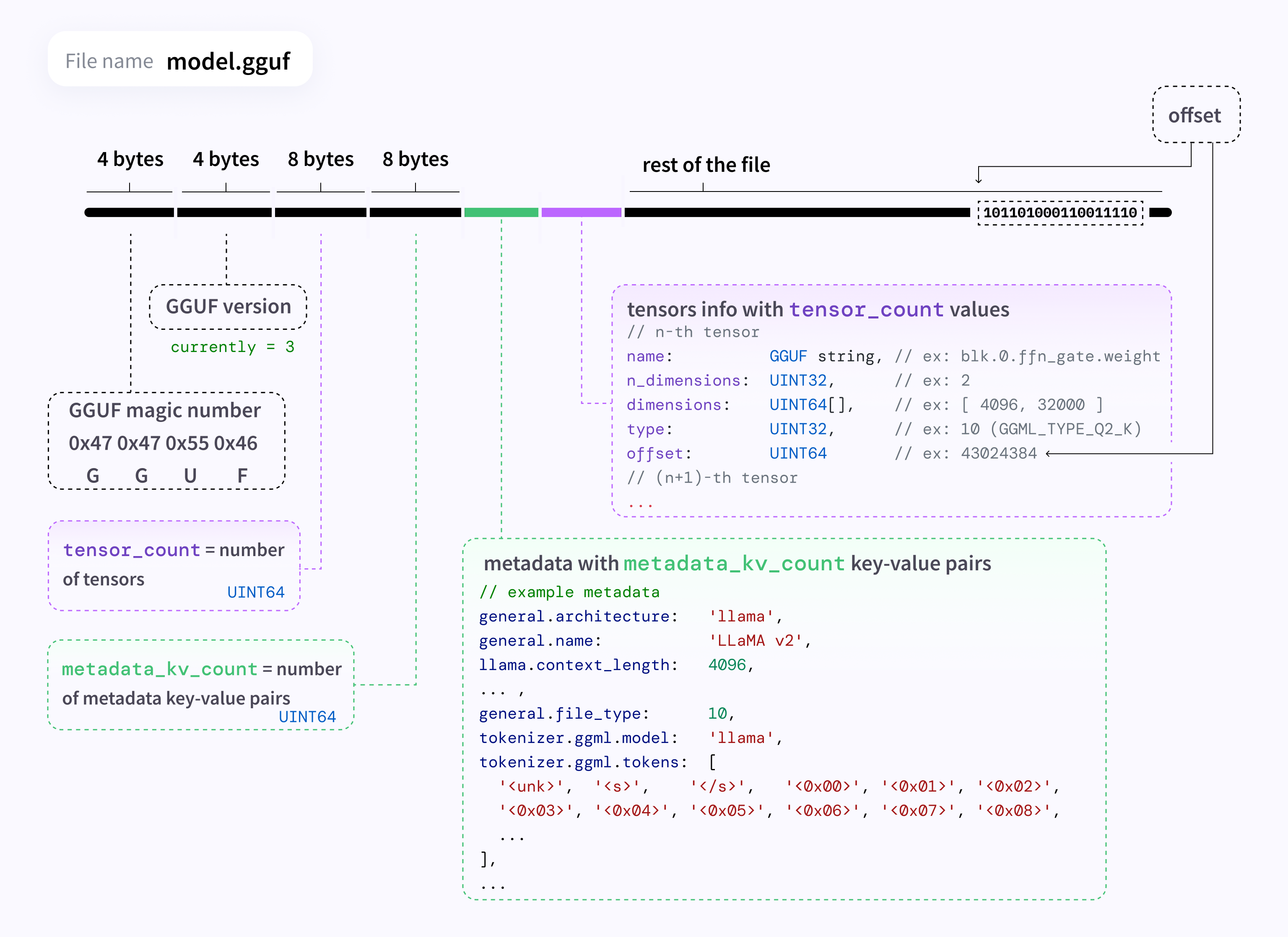
As a summary of the advantages of the GGUF format:
Smaller file sizes compared to other formats.
Faster loading times.
Improved cross-platform compatibility.
Rich built-in support for different quantization levels.
One of the most important features in GGUF is its quantization setups. These span across various settings and configurations, from high-level legacy quants that are applied equally to each weight, up to low-level customizable quants, where specific weights in a layer could be quantized differently or with mixed precision.
In the following section, I’ll go through the GGUF quantization types, providing a short description with bullet points for each type, as this is a low-level, advanced concept that an AI Engineer probably won’t work too much on.
If you want to dive into the nits & bits of quant types, check this Table.
2. What Quantizations does GGUF Support?
When working with any GGUF model, you might see the model name has a suffix attached, such as Q4, Q5_K, IQ2_K_S, etc. Each of these names stands for an identifier of what type and class of quantization the model was compressed and stored as.
Tip: The next section dives deep into Floating Point precision and maths, feel free to skip it.
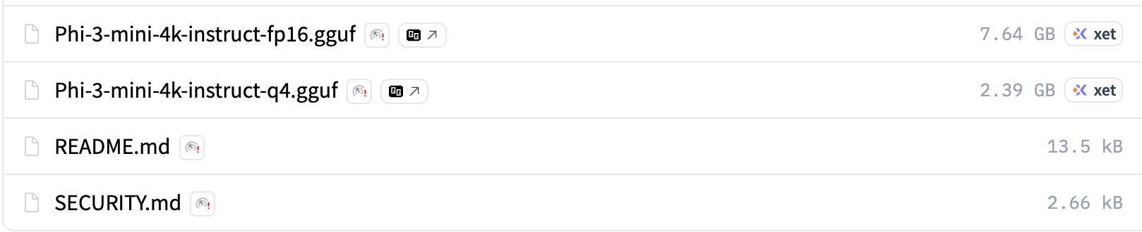
Let’s take the `microsoft/Phi-3-mini-4k-instruct` model as an example. It comes in 2 variants, an FP16 non-quant, and a Q4 GGUF quant.
That means that for FP16, each `weight` is represented in 16 bits:
Whereas for Q4, each `weight` is represented in 4 bits, but with a trick:
All 4 bits store an integer code, no separate sign/exponent/mantissa in those 4 bits, we’ll call this QuantizedWeight.
Instead, a shared scale is stored per block of weights, let’s call it SharedScale.
The real value of each weight is reconstructed during inference as
Weight = SharedScale * QuantizedWeightBut first, why does GGUF have so many quant variations?
The main reason is that some layers, such as those for EMB (embeddings), are very sensitive to precision loss, whereas other layers as some FFN (feed forward ones), can be heavily quantized with minimal effect on outputs.
Tip: The key goal here is to customize and squeeze the most quality out of the model, while keeping its memory and compute footprint as low as possible.
Let’s take the`Q4_K_S` variant as an example, and unpack what that means:
Q stands for Quantization.
The digit 4 stands for the number of bits the weights are quantized in.
K shows that the layers of the model were quantized in a block-wise structure. The layer weights are split into blocks, and each of the blocks is quantized using a different factor for that block.
S/M/L is a block size, and it helps determine the tradeoff between accuracy and compression. Larger blocks = more compression = lower accuracy.
Although there are many configurations, we can generally split the quants into 3 distinct groups: Legacy, K-Quants, and I-Quants, ordered from the oldest to the newest added.
Legacy Quants (Q4_0, Q4_1, Q8_0)
These are block quantization: the layer’s weights are divided into fixed-size blocks.
Uses one (
_0) or two (_1) extra constants per block, to scale weight values back from their quantized value.Fast and straightforward, but less precise than modern methods.
K-Quants (Q3_K_S, Q5_K_M)
A K quant is a block-wise quantization, with weights split into blocks and scaled with per-block factors.
These also support mixed quantization, where some layers could be compressed more in order to give more bits to critical layers.
I-Quants (IQ2_XXS, IQ3_S)
In simple terms, an I quant builds on top of a K quant, introduces an Importance Matrix with lookup tables to preserve critical weights.
An importance matrix is basically used to identify which weights carry more value for the model output quality, such that the weight is quantized less, whereas the “less important” weights are quantized more.
Best for memory-limited environments with sufficient compute power.
A large majority of GGUF models are quantized with K Quants or I Quants, especially for the larger models, which makes sense as they require more optimizations to reduce the memory footprint.
Tip: Learn more about Quants only if you want to deploy LLMs on resource-constrained hardware.
At this point, we already have an understanding of what GGUF is and how LLM checkpoints are quantized and stored in the GGUF format.
To complete the core picture, we need to further understand how `llama.cpp` loads, parses, and interprets a GGUF model.
So, let’s get into the good stuff!
3. What is GGML? (tl;dr)
tl;dr: ggml [1] is a machine learning (ML) library written in C and C++ with a focus on Transformer inference. ggml is similar to ML libraries such as PyTorch and TensorFlow.
So, GGML [1] is the actual backbone, the core library that provides and executes all the tensor operations and provides all the optimizations necessary for high-performance computation.

An equally important detail to note about GGML is its extensibility and portability.
As it’s written in C++, GGML (and llama.cpp) can be compiled for virtually any hardware platform, from x86_64 (AMD/Intel) to ARM64 (M1, M2, M3), and other architectures.
The primary hardware target is the CPU, as GGML supports SIMD (Single Instruction Multiple Data) for newer CPUs, which in short means parallel computation leveraging the CPU’s multi-core threading.
That was for the CPU, on the GPU side - it also supports accelerators such as `ggml-cuda` and `ggml-metal`. These accelerators enable llama.cpp to execute the GGML computation graph on GPU hardware, by basically translating the instructions to the GPU’s own “language” which for CUDA is PTX, and for Apple is Metal.
Note: But all those details might be interesting for a Compiler or Deep Learning Engineer, we are AI/ML Engineers.
Given that, let’s conclude what’s powerful about GGML:
Can be compiled to multiple architectures (arm64, x64, x86)
It’s an ML Library, similar to PyTorch or Tensorflow
Runs fast on CPUs, but also supports GPU accelerators.
It’s the core of llama.cpp, executing all the tensor operations.
Now we’ve learned that GGUF is the format of storing the model weights, and GGML is the actual Tensor Library that parses, loads, and executes the LLM model.
The third and last missing piece is llama.cpp and how everything fits together. We’ll cover that next.
4. The Llama.cpp Library Workflow
Note: For the writing and diagrams of this section, I’ve analyzed the llama.cpp codebase, official discussion threads, closed/open PRs, and trusted resources.
First off, I have to say - the llama.cpp codebase is enormous.
If we were to unpack everything, that’s a book ready to be published already. Our focus is different.
“We’ll leave the complex details to the code owners. We care about how it works.”
And to get there, we’ll cover only 4 components at a high level that make the entire workflow just click.
Model Loading → parsing GGUF, loading config, architecture, etc.
Populating Weights → how the execution graph is compiled for inference.
KV Cache Handling → how KV cache is handled during inference.
Token Sampling → how a token gets selected from the distribution.
Let’s start with them in order.
1. GGML Model Loading
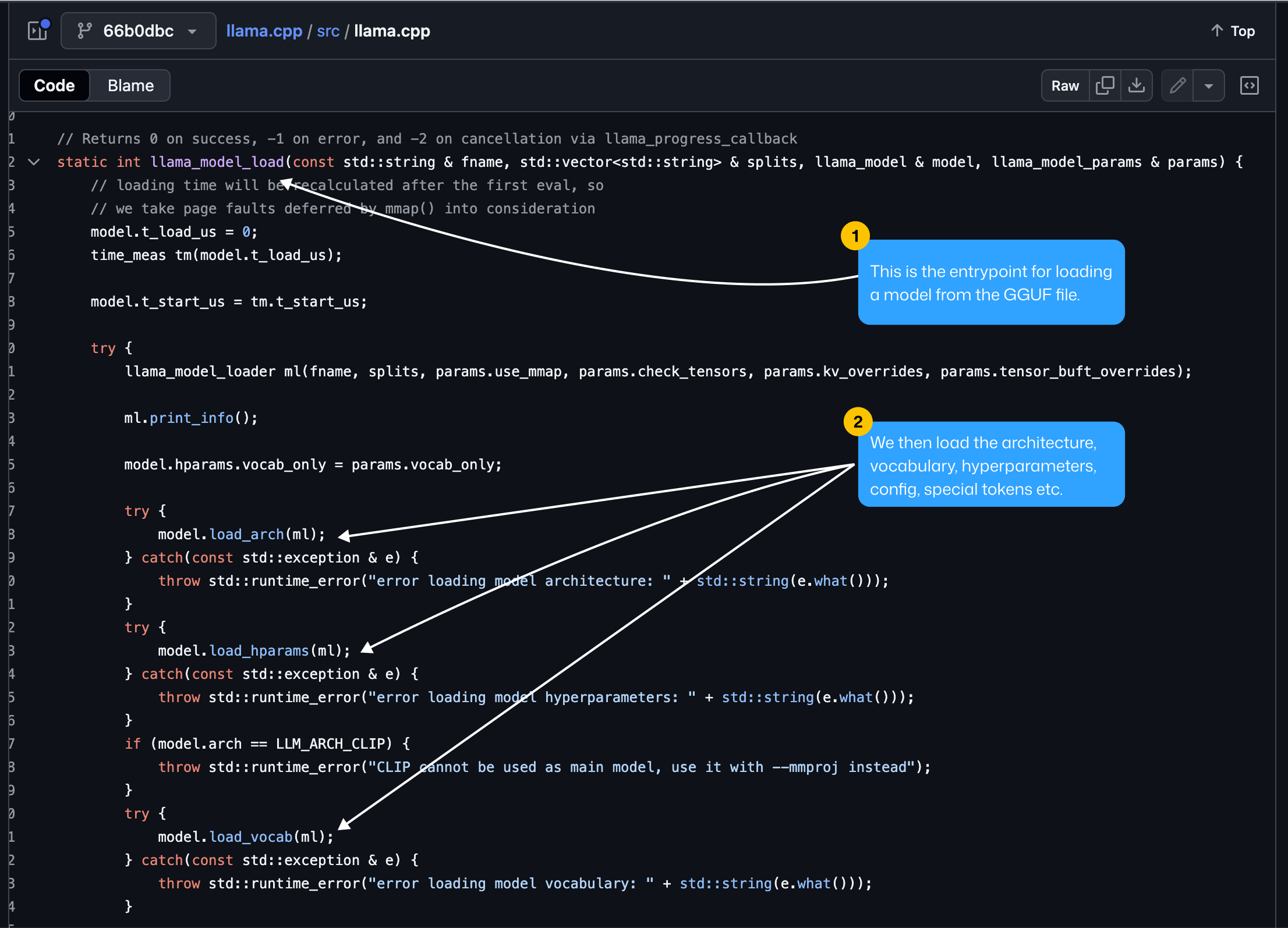
After defining the model architecture type, which is usually inferred from the GGUF metadata fields, the next step is to start defining the execution graph of the model, as after this step, we’ll be able to load weights for each tensor.
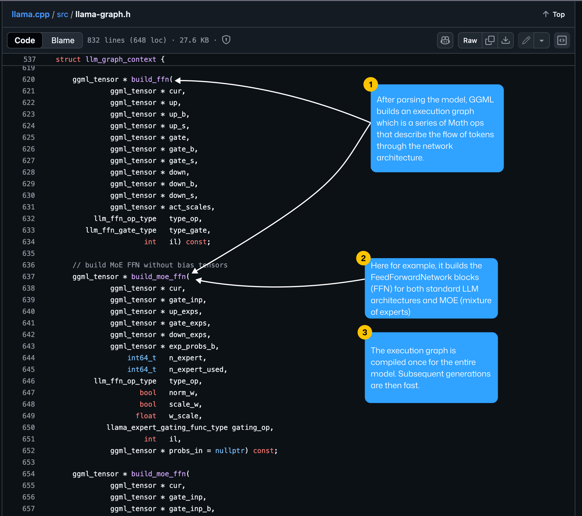
2. GGML Populating Weights
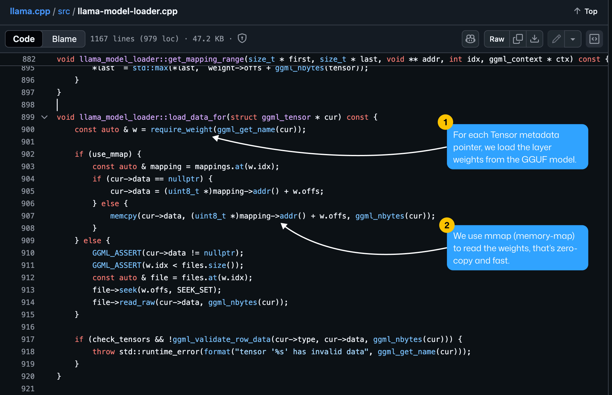
For each layer within the model graph, we’re loading the weights from the GGUF file using `mmap`, or Memory Mapping.
Def: mmap is a POSIX-compliant Unix system call that maps files or devices into memory. It is a method of memory-mapped file I/O.
This approach allows the model to access weight data without fully loading it into RAM, enabling efficient, on-demand retrieval from disk.
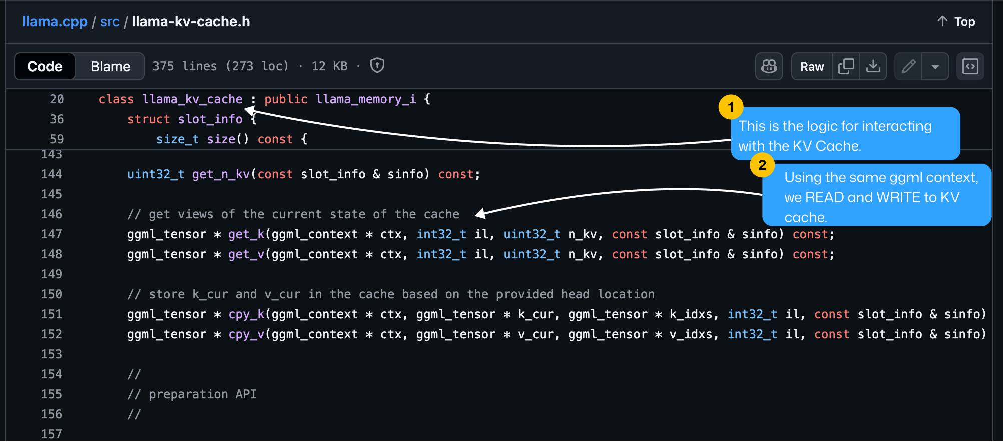
3. GGML KV Cache Handling
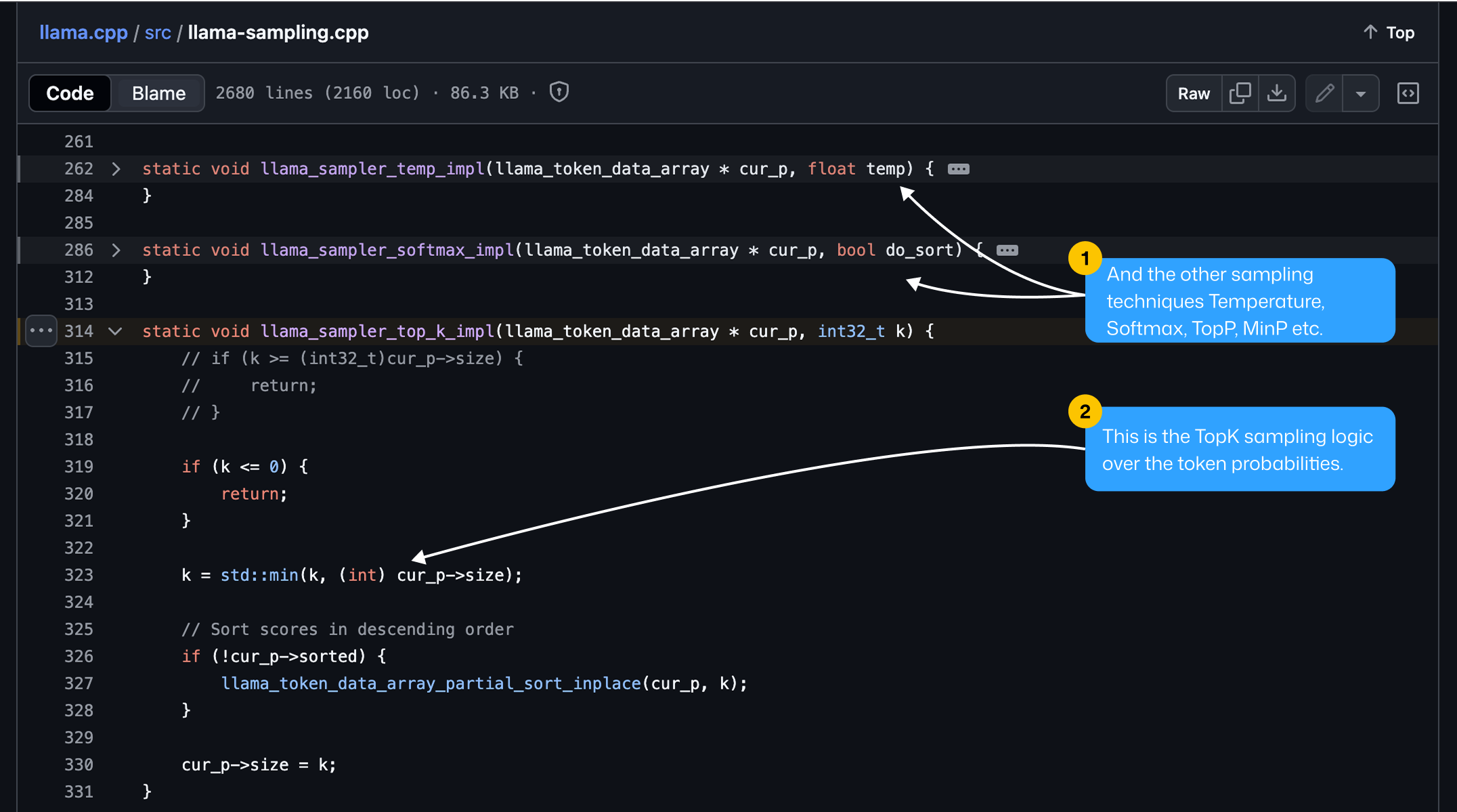
4. GGML Token Sampling
5. The High-Level Architecture
The succession of steps in llama.cpp [2], is to load the model architecture, define the execution graph, and populate weights for each tensor in the graph. Further, the model is ready for inference, and the last two steps from those described above come into place during LLM, generating a new token.
Tip: For a complete understanding on how LLMs generate tokens, read this [10].
Now, after going through all the core steps and their order, we can finally represent everything as a complete workflow in the sequence diagram below.
To solidify our understanding one last time, we have this workflow to describe the end-to-end template of how llama.cpp, GGML, and GGUF come in together:
The GGUF model is loaded by llama.cpp
The GGUF binary file is parsed, and GGML allocates placeholders for tensors.
Then the execution graph of the LLM model is constructed.
Next, we load the weights for each tensor in the graph.
At this point, the model is ready for inference.
The user sends an input prompt.
The prompt is tokenized, and token_ids are passed through the model.
The Model graph is executed with initial tokens.
The KV Cache state for the initial iteration is saved.
A new token is sampled from the probability distribution of the vocabulary.
The new sampled token is detokenized and streamed to the client.
The updated sequence (initial + new token) is passed through the graph loop.
After finishing the generation, we release the memory buffers.
The user gets the final output text.
5. [BONUS] Live Code on inspecting GGUFs
The tl;dr for this following 20min tutorial covers:
Downloading models using huggingface-cli
Setting up Rust and Cargo, installing`safetensors_explorer`
Inspecting a GGUF model from your Terminal
Generating HF Access Token, explaining Token Types
Explaining each data entry in the GGUF model
Explaining why some layers are FP32, whereas others are Q4
Hands-on coding, plus rich key details along the way
6. Conclusion
In this article, we’ve learned the most popular stack of running LLMs on resource-limited hardware, CPUs, and Edge Devices. Multiple options allow you to deploy models locally, and all of them are powered by llama.cpp, with the best example being Ollama, which has over 150k stars.
And that actually connects with the upcoming article, as we’ll be covering Ollama, but with more hands-on coding, and practical tips you could apply to your own projects and systems.
We’ve covered the core components of llama.cpp: GGUF and GGML, with GGUF being an actively adopted format seen in other frameworks such as vLLM.
For AI engineers, learning about Edge AI is one of the most strategic moves you can make today. AI shows signs (OSS, smaller models, etc.) of increasingly moving towards processing data closer to where it’s generated.
Understanding how to optimize models for local and edge deployment will position you strongly for the coming years. This may not happen in the next year, but investing in this knowledge now will give you a significant upper hand.
Hope you enjoyed this article!
Images and Media were generated by the author, if not otherwise stated.
References
[1] Introduction to ggml. (2025, February 24). Huggingface.co. https://huggingface.co/blog/introduction-to-ggml
[2] ggml-org/llama.cpp: LLM inference in C/C++. (2025). GitHub. https://github.com/ggml-org/llama.cpp
[3] LLM Visualization. (2025). Bbycroft.net. https://bbycroft.net/llm
[4] Edge AI Market Size, Share & Growth | Industry Report, 2030. (2024). Grandviewresearch.com. https://www.grandviewresearch.com/industry-analysis/edge-ai-market-report
[5] GGUF. (2025). Huggingface.co. https://huggingface.co/docs/hub/en/gguf
[6] GGUF - vLLM. (2025). Vllm.ai. https://docs.vllm.ai/en/stable/features/quantization/gguf.html
[7] Nscale Contracts Approximately 200,000 NVIDIA GB300 GPUs with Microsoft to Deliver NVIDIA AI Infrastructure Across Europe and the U.S. | Press Release | Nscale. (2025). Nscale.com. https://www.nscale.com/press-releases/nscale-microsoft-2025
[8] Colossus | xAI. (2024). X.ai. https://x.ai/colossus
[9] Helix: A Vision-Language-Action Model for Generalist Humanoid Control. (2025, February 20). FigureAI. https://www.figure.ai/news/helix
[10] Razvant, A. (2025, February 20). Understanding LLM Inference. Substack.com; Neural Bits. https://multimodalai.substack.com/p/understanding-llm-inference
