Understanding LLM Optimization Techniques

Weights quantization using GPTQ, BitsAndBytes. Parallelism techniques, KV-caching, Flash Attention and Speculative Decoding.

In this article, you’ll learn about:

• LLM Quantization

• How to use GPTQ and BitsAndBytes

• Pipeline/Tensor/Sequence Parallelism

• KV-Cache, Flash Attention

• Static, Dynamic, Continuous LLM Requests Batching

• Speculative Decoding using large/small pair LLMs

---

This article will discuss optimizations that can be applied to the Model, Compute, and Serving contexts of deploying LLMs into production.

Figure 1. The optimization techniques we presented in this article. Contains images from [3], [4], [5], [6]

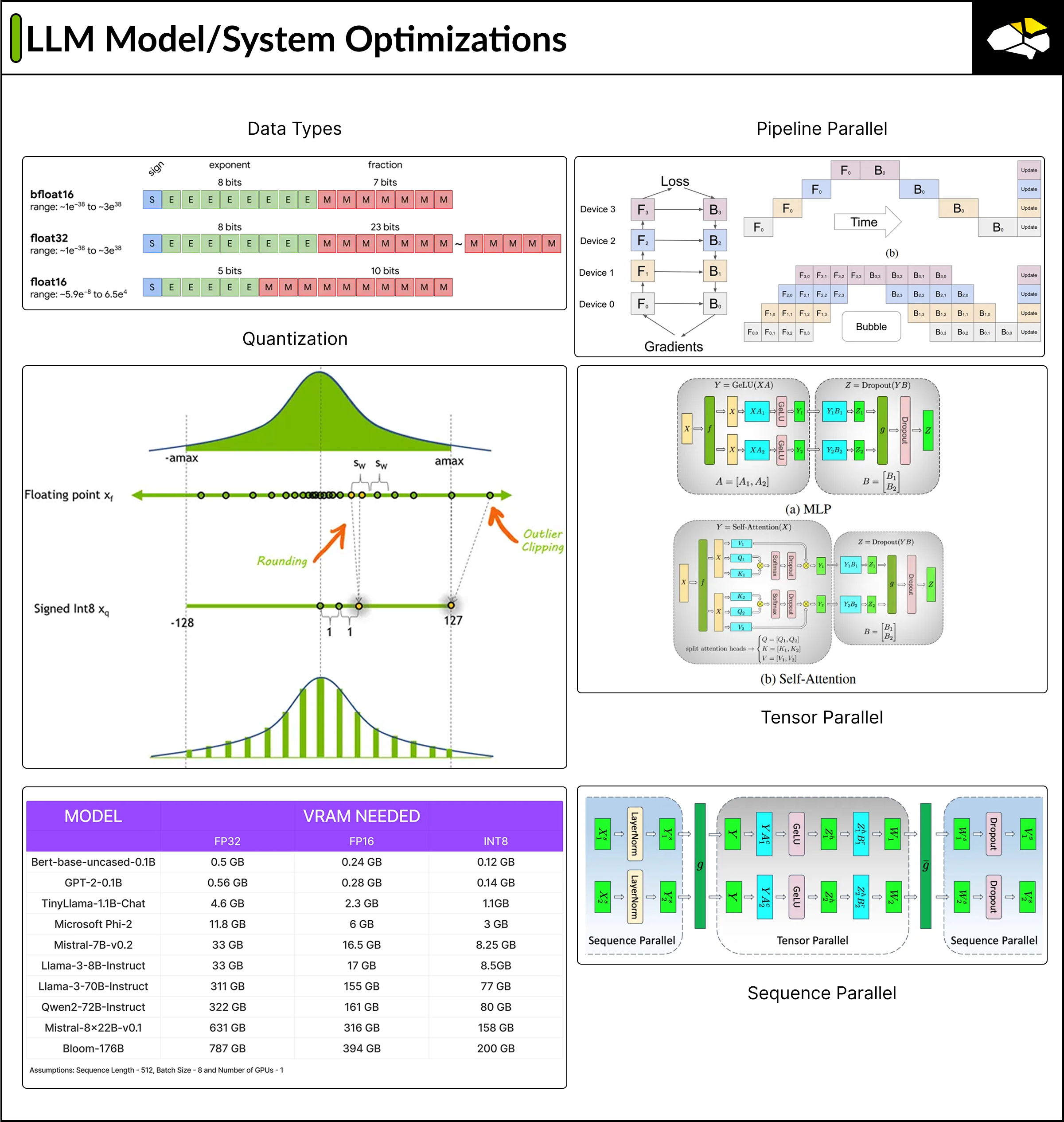
We’ll cover Quantization using BitsAndBytes and GPTQ, Sparsity, and Knowledge Transfer as the first layer of optimizations we can apply to the LLM model.

Then, we’ll cover parallelization techniques such as Model, Tensor, and Sequence, which allow us to partition and spread the inference execution across multiple devices. These techniques are largely used in inference deployments of large LLM models.

Finally, we’ll cover request batching, KV-caching, Flash Attention, and Speculative decoding to further speed up the throughput during inference.

---

Table of Contents

1. Recap on Prefill/Decode LLM Inference Phases

2. Model Optimization Techniques

   1. DataTypes (FP32/FP16/BF16)

   2. Quantization, Sparsity

   3. BitsAndBytes, GPTQ

   4. Knowledge Transfer Finetuning

3. Parallelisation Optimization Techniques

   1. Model/Tensor/Pipeline Parallelism

4. Model Serving Optimizations

   1. Static, Dynamic, and Continuous Batching

   2. KV-Caching

   3. Flash Attention

   4. Speculative Decoding

5. Conclusion

---

The previous article on LLM Inference taught us that LLMs are auto-regressive and generate outputs one token at a time. The inference process is split into two stages: Prefill and Decode. For a short recap, please see the following article:

Understanding LLM Inference

To extract the key details from the article, we get these insights:

1. Prefill phase runs fast because LLMs know the entire context of the input, and operations can be parallelized, leading to efficient use of the GPU.

2. On the other hand, Decode is memory-bound as it generates one token at a time. Thus, the GPU is used sub-optimally.

There are a few ways to remediate this problem, and many of these techniques have already been implemented in popular LLM serving frameworks.

Performance optimizations can be divided into model-based and process-based ones. Model-based ones refer to changes and optimizations directly applied to the LLM model, such as quantization, pruning, and distillation.

Process-based optimizations would apply to the inference flow, covering batching, KV-Cache, Model/Tensor/Pipeline parallelism, Flash Attention, and Speculative Decoding.

---

Model Optimizations

When discussing optimizing LLM models or any Deep Learning model, we refer to transformations that could be applied internally to increase the throughput performance without a significant loss in accuracy.

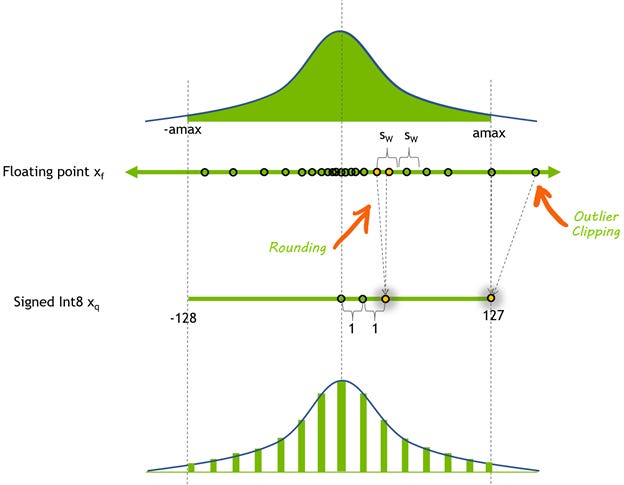
One of the first optimizations that ML Engineers look into is weight precision quantization. This transformation is a model compression technique that converts the weights and activations within an LLM from higher precision, by default FP32/FP16, to lower precision, such as INT8 or INT4.

Most LLM models are trained in BF16 precision.

Because LLMs have Billions of parameters, loading them into memory in their default format would require lots of GPU memory, which is not accessible to anyone.

Figure 1. Data Types structure, FP32, FP16, BF16. Taken from [1]

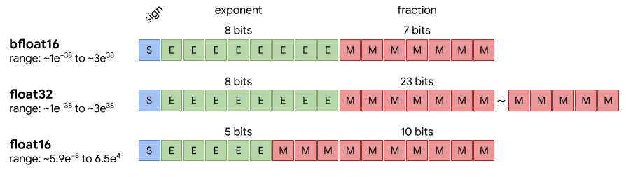
1. FP32 (8bits exponent, 23 bits mantissa) (31bits + 1 for sign)

   1. Although not many LLM models are trained in full FP32 precision, a mixed FP32 + BF16 might be used to maintain gradient stability during training.

2. FP16 (5bits exponent, 10bits mantissa) (15bits + 1 for sign)

   1. This is the half-precision format.

3. BF16 (8bits exponent, 7bits mantissa) (15bits + 1 for sign)

   1. This format was developed by Google and was called Brain Floating Point Format, or BFloat for short. BF16's main advantage is that it can represent some extremely high values that FP16 cannot, which matters during training. This is possible due to more exponent bits.

The idea behind using a higher precision format when training is that, due to the large dataset size, we want it to encode in its weights the most intricate information of its latent space where tokens are. The more mantissa bits, the more specific the model can learn where to map the tokes from the training set in the embedding space.

Higher precision is key during training. We can quantize to lower precision during inference to make the model run efficiently. The less memory used, the higher the parallelism we can achieve, thus increasing performance.

Quantization solves the main problem of the VRAM requirement. The following image shows rough approximations of how much GPU Memory we would require for each format.

Source: https://blog.runpod.io/understanding-vram-and-how-much-your-llm-needs

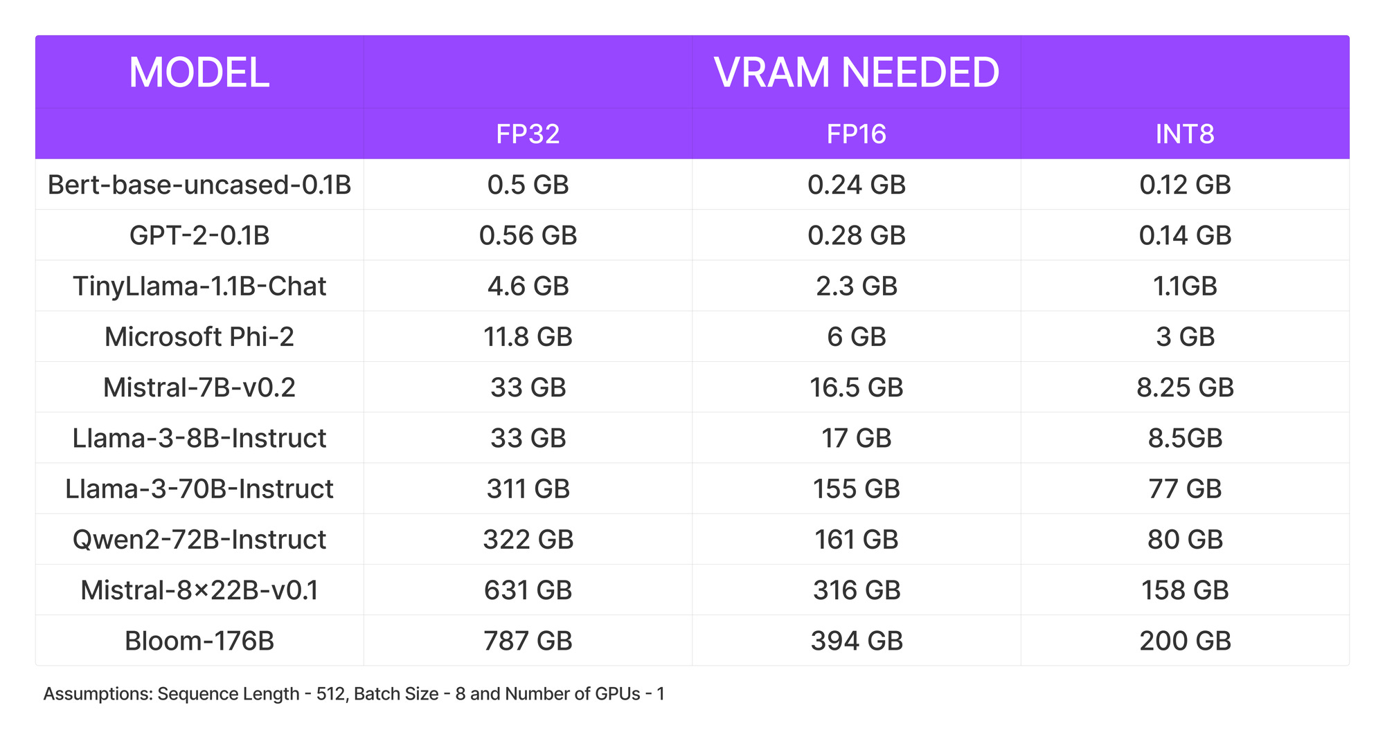
ℹ️ Quantization works especially well for text generation since all we care about is choosing the set of most likely next tokens and don’t really care about the exact values of the next token logit distribution.

All that matters is that the next token logit distribution stays roughly the same so that an argmax or topk operation gives the same results.

How to quantize an LLM?

There are 2 popular libraries we can use: BitsAndBytes and GPTQ.

Figure 2. 8-bit signed Integer quantization for a floating point X tensor. Taken from [9]

BitsAndBytes

The bitsandbytes library is a lightweight Python wrapper around CUDA custom functions, particularly 8-bit optimizers, matrix multiplication (LLM.int8()), and 8- and 4-bit quantization functions. It is the easiest option for quantizing a model to 8- and 4-bit precision.

How does it work?
8-bit quantization multiplies outliers in fp16 with non-outliers in int8, converts the non-outlier values back to fp16, and then adds them together to return the weights in fp16.

This reduces the degradative effect outlier values have on a model’s performance. 4-bit quantization compresses a model even further, and it is commonly used with QLoRA to finetune quantized LLMs.

pip install bitsandbytes

from transformers import AutoModelForCausalLM, BitsAndBytesConfig

quantization_config = BitsAndBytesConfig(load_in_8bit=True)

model_8bit = AutoModelForCausalLM.from_pretrained(
    "bigscience/bloom-1b7", 
    quantization_config=quantization_config
)

The BitsAndBytesConfig could take one or multiple arguments from this set:

• load_in_8bit

  • Enables 8-bit quantization with LLM.int8().

• load_in_4bit

  • Enables 4-bit quantization using FP4/NF4 layers from bitsandbytes.

• llm_int8_threshold

  • Sets the outlier threshold for outlier detection in LLM.int8(), determining which values are processed in fp16.

• llm_int8_skip_modules

  • An explicit list of modules to exclude from 8-bit conversion.

• llm_int8_enable_fp32_cpu_offload

  • Enables splitting the model to run int8 on GPU and fp32 on CPU.

• llm_int8_has_fp16_weight

  • Runs LLM.int8() with 16-bit main weights, useful for fine-tuning.

• bnb_4bit_compute_dtype

  • Sets the computational data type, which can differ from the input type.

• bnb_4bit_quant_type

  • Sets the quantization data type in bnb.nn.Linear 4Bit layers (FP4 or NF4).

• bnb_4bit_use_double_quant

  • Enables nested quantization of quantization constants.

• bnb_4bit_quant_storage

  • Sets the storage type for quantized 4-bit parameters.

GPTQ

GPTQ is a post-training quantization (PTQ) method that makes the model smaller with a calibration dataset.

The idea behind GPTQ is very simple: It quantizes each weight by finding a compressed version that yields a minimum mean squared error. The GPTQ algorithm requires calibrating the quantized weights of the model by making inferences about the quantized model.

pip install --upgrade accelerate optimum transformers 
pip install gptqmodel --no-build-isolation

import torch
from transformers import AutoModelForCausalLM, AutoTokenizer, GPTQConfig

quantizer = GPTQQuantizer(bits=4, dataset=dataset_id, model_seqlen=2048)
quantizer.quant_method = "gptq"
dataset_id = "wikitext2"
model_id = "meta-llama/Meta-Llama-3-8B"

model = AutoModelForCausalLM.from_pretrained(model_id, config=quantizer, torch_dtype=torch.float16, max_memory = {0: "15GIB", 1: "15GIB"})
tokenizer = AutoTokenizer.from_pretrained(model_id, use_fast=False)

examples = [
    tokenizer("Patient presented with persistent cough and fever."),
    tokenizer("MRI showed no signs of acute stroke."),
    tokenizer("Administered 5mg of ibuprofen for pain management.")
]  
model.quantize(examples)

quantized_model_dir = "llama38b_gptq_q4b_slen2048"
model.save_quantized(quantized_model_dir)

Sparsity

Like quantization, many deep learning models are robust to pruning or replacing certain values close to 0 with 0. Sparse matrices are matrices in which many of the elements are 0. They can be expressed in a condensed form that takes up less space than a full, dense matrix.

Figure 3. Weights sparsity analysis for Llama 7B model and the relationship to VRAM requirements. Taken from [8]

Sparse models require less storage memory, as many weights are zero and can be efficiently compressed.

The lower memory requirements translate into reduced data transfer costs, especially in cloud-based applications, making LLMs more accessible and cost-effective for a broader range of users and applications.

Knowledge Transfer

Another approach to shrinking the model size is distilling a larger model’s knowledge into a smaller, task-specific model. This concept, which dates back to 2015 with the Knowledge Distillation for Neural Networks paper, is a form of knowledge distillation. The common practice is to have a bigger, more performant model generate a curated dataset of samples to fine-tune a smaller task-specific model.

One of the most recent examples of successfully using knowledge transfer is DeepSeek R1/R1-Zero reasoning models, where larger models 670B were trained using RL and then used to produce a small set of engineered CoT prompts that were used to train smaller 3B-70B models, which did very well in benchmarks.

Figure 4. DeepSeek R1 and Distilled variants performance on benchmarks. Taken from [3]

Parallelization Optimizations

One way to reduce the per-device memory footprint of the model weights is to distribute the model over several GPUs. This enables the running of larger models or batches of inputs. Based on how the model weights are split, there are three common ways of parallelizing the model: pipeline, sequence, and tensor.

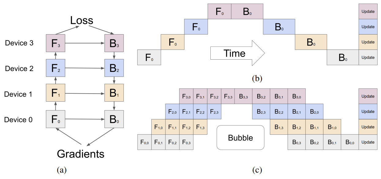
Pipeline parallelism

Pipeline parallelism involves sharding the model (vertically) into chunks, each comprising a subset of layers executed on a separate device. Thus, each device's memory requirement for storing model weights is effectively quartered.

Limitation: Because this execution flow is sequential, some devices may remain IDLE while waiting for the output of the previous layers.

Figure 5. Illustration of Pipeline Parallel showcasing mini-batch passes through the partitioned model. Taken from [5]

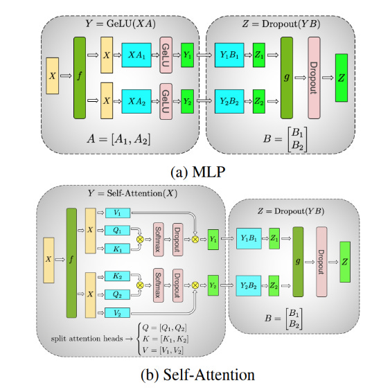
Tensor parallelism

Tensor parallelism involves sharding (horizontally) individual layers of the model into smaller, independent blocks of computation that can be executed on different devices.

In transformer models, the Attention Blocks and MLP (normalization) layers will benefit from Tensor Parallelism because large LLMs have multiple Attention Heads. To speed up the computation of Attention Matrices, which is done independently and in parallel, we could split them into one per device.

Figure 6. Illustration of tensor parallelism in multi-layer perceptron (MLP) and self-attention layers. Taken from [6]

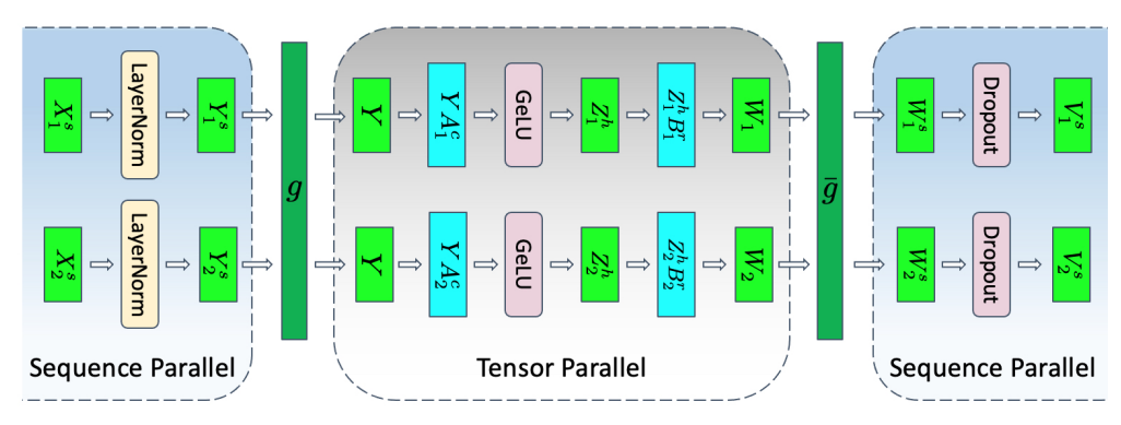
Sequence Parallelism

Tensor parallelism has limitations. It requires layers to be divided into independent, manageable blocks. This does not apply to operations like LayerNorm and Dropout, which are replicated across the tensor-parallel group. These layers are computationally inexpensive but require considerable memory to store activations.

To mitigate this bottleneck, sequence parallelism partitions these operations along the “sequence dimension” where the Tensor Parallelised layers are, making them memory efficient.

Figure 7. An illustration of a transformer layer using both tensor and sequence parallelism. Taken from [7]

Techniques for model parallelism are not exclusive and can be used in conjunction.

Serving Optimizations

This section discusses request batching and KV caching, common optimization techniques already built into various LLM model-serving frameworks, such as TGI, vLLM, TensorRT-LLM, or Ollama.

Request Batching

Source: https://www.baseten.co/blog/continuous-vs-dynamic-batching-for-ai-inference/

The simplest batching strategy is “static batching,” which involves creating fixed batches of requests before the processing starts. This method is naive for LLMs and doesn’t work, mainly because LLMs generate only one output token at a time.

For example, if we set a batch-size=2 and pass in the following prompts to our LLM:

P1 : Write a short 10 words story about computers
P2 : Write an essay of 500 words about computers.

It makes sense to get the response of P1 faster, as the generated text is 10 words long compared to 500 words of P2. In this case, we’ll get a response only when the longest request has finished. They’ll have different processing times, with P2 taking the longest.

Dynamic Batching

Compared with static batching, dynamic batching adds elasticity, which we can configure using 2 parameters:

1. A maximum batch size

2. A window to wait after receiving the first request before running a partial batch.

A batch will be processed once the maximum batch size is exceeded or the time window we set is exceeded without any new incoming requests. In the following example, let’s visualize how the dynamic batching mechanism runs:

• In the first example, max-batch-size = 4, and we’ve got 3 incoming requests until the time window of 10ms has passed. We ran inference on a batch of 3

• In the second example, max-batch-size = 4, we received 4 requests within the time window. Since we reached max-batch-size, we ran inference on a batch of 4.

[MaxBatch=4][T=10ms] (time window passed no new requests)
Request: --R1-------R2-----------------------R3--|
Process: --|-(wait)-|-(wait)-----------------| -> exec (bs=3)
Time:    --|10-9-8--|-10-9-8-7-6-5-4-3-2-1|-----------

[MaxBatch=4][T=10ms] (max batch size reached)
Request: --R1----------R2---------R3---------R4--|
Process: --|-(wait)----|-(wait)---|-(wait)---|-> exec (bs=4)
Time:    --|-10-9-8-7--|-10-9-8-7-|-10-9-8-7-|-10-9-8--|

Dynamic batching is great for live traffic on models like Text2Image because the diffusion process of generating an image from text takes roughly the same, regardless of text description size.

For LLMs, however, even if we batch multiple requests together, we’ll still have to wait for the longest one in the batch to complete before getting a response. This leaves GPU resources idle.

The specific batching strategy for LLMs is Continuous Batching.

Continuous Batching (Iteration Batching)

Continuous batching can be considered a variation of Dynamic Batching, only that it works at the token level instead of the request level. For continuous batching, a layer of the model is applied to the next token of each request.

In this manner, the same model weights could generate the N’th token of one response and the Nx100 token of another. Once a sequence in a batch has completed generation, a new sequence can be inserted in its place, yielding higher GPU utilization than static batching.

Source: https://friendli.ai/blog/llm-iteration-batching

The continuous batching technique was initially introduced under the “iteration-level-scheduling” term from the 2022 Orca: A Distributed Serving System for Transformer-Based Generative Models paper.

Since the prefill phase takes compute and has a different computational pattern than generation, it cannot be easily batched with the generation of tokens.

Continuous batching frameworks currently manage this via hyperparameter: waiting_served_ratio, or the ratio of requests waiting for prefill to those waiting end-of-sequence tokens.

KV Caching

One common optimization for the decode phase is KV caching. The decode phase generates a single token at each time step. Still, each token depends on all previous tokens' key and value tensors (including the input tokens’ KV tensors computed at prefill and any new KV tensors computed until the current time step).

To avoid recomputing all these tensors for all tokens at each time step, it’s possible to cache them in GPU memory.

Source: https://developer.nvidia.com/blog/mastering-llm-techniques-inference-optimization/

Flash Attention

Flash attention is an optimized kernel that fuses layer operations to avoid frequent RW operations from the GPU memory.

On GPUs, we have High Bandwidth Memory (HBM), which is large in memory but slow in processing. The standard Attention mechanism processes K, Q, and V on HMB, and frequent reads/writes become a bottleneck.

On the other hand, SRAM (Static Random Access Memory) is fast in operations but smaller in memory.

Flash Attention loads the K, Q, and V once. Then, it uses a fused attention CUDA kernel to compute the attention matrices and write them back to HBM.

Source: https://huggingface.co/docs/text-generation-inference/en/conceptual/flash_attention

Speculative Decoding

When generating tokens, LLMs predict a probability distribution from which we sample the next token. In standard decoding, each token is sampled during a forward pass of logits through the last linear and softmax layer of the LLM model.

Speculative decoding aims to " advance” a few candidate tokens using a smaller model and then select the best candidate to include in the sequence.

# Notations: 
# bLLM (bigLLM)| sLLM (smallLLM)
# bTok (bigLLM Tokenizer) | sTok (smallLLM Tokenizer)

------
code>
------
def speculative_decoding(sLLM, bLLM, sTok, bTok, prompt, max_toks=50):
    
    # Step 1: Generate draft using Small Model
    inputs = sTok(prompt, return_tensors='pt').to(device)
    s_outs = sLLM.generate(inputs['input_ids'], max_new_tokens=max_toks)
    draft = sTok.decode(s_outs[0], skip_special_tokens=True)

    # Step 2: Verify the draft with the big model
    big_inputs = bTok(draft, return_tensors='pt').to(device)

    # Step 3: Calculate log-likelihood of the draft tokens under bLLM
    with torch.no_grad():
        outputs = bLLM(big_inputs['input_ids'])
        log_probs = torch.log_softmax(outputs.logits, dim=-1)

    draft_token_ids = big_inputs['input_ids']
    log_likelihood = 0
    for i in range(draft_token_ids.size(1) - 1):
        token_id = draft_token_ids[0, i + 1]
        log_likelihood += log_probs[0, i, token_id].item()

    avg_log_likelihood = log_likelihood / (draft_token_ids.size(1) - 1)
    return draft, avg_log_likelihood

Then, based on the average_log_likelihood the draft is added to our initial sequence. In the following animation from GoogleResearch we can see speculative decoding in action.

See DataCamp tutorial for a hands-on deeper dive into speculative decoding.

Conclusion

This article covered LLM model quantization, pruning, and knowledge transfer as model optimizations. We also presented parallelism techniques such as pipeline, tensor, and sequence parallel to speed up the inference and throughput of deployed LLM models.

We’ve provided code samples to demonstrate quantization using GPTQ and BitsAndBytes, and implemented a draft speculative decoding flow using 2 LLM models working side by side.

This article gives you a broad overview of the LLM Inference Optimization techniques ML Engineers can use to increase the throughput of LLMs deployed to production environments.

---

References:

[1] Google Cloud, Improve your model’s performance with bfloat16. (2019)
https://cloud.google.com/tpu/docs/bfloat16

[2] Datacamp. Quantization for Large Language Models (LLMs) (2024)
https://www.datacamp.com/tutorial/quantization-for-large-language-models

[3] DeepSeek R1 deepseek-ai/DeepSeek-R1 GitHub (2024)
https://github.com/deepseek-ai/DeepSeek-R1

[4] LLM Quantization | GPTQ | QAT | AWQ | GGUF | GGML | PTQ (2024)
https://medium.com/@siddharth.vij10/llm-quantization-gptq-qat-awq-gguf-ggml-ptq-2e172cd1b3b5

[5] Google, GPipe: Easy Scaling with Micro-Batch Pipeline Parallelism (2019)
https://arxiv.org/pdf/1811.06965.pdf

[6] Nvidia, Megatron-LM: Training Multi-Billion Parameter Language (2020)
https://arxiv.org/pdf/1909.08053.pdf

[7] Nvidia, Reducing Activation Recomputation in Large Transformer Models (2022)
https://arxiv.org/pdf/2205.05198.pdf

[8] NeuralMagic, Why is Sparsity Important for LLMs?
https://docs.neuralmagic.com/llms/guides/why-weight-sparsity/

[9] Nvidia. Achieving FP32 Accuracy for INT8 Inference Using Quantization Aware Training with NVIDIA TensorRT https://developer.nvidia.com/blog/achieving-fp32-accuracy-for-int8-inference-using-quantization-aware-training-with-tensorrt/