

Complete Overview in Vision AI 2025
From Pixels to Vision Language Models. Updated periodically.

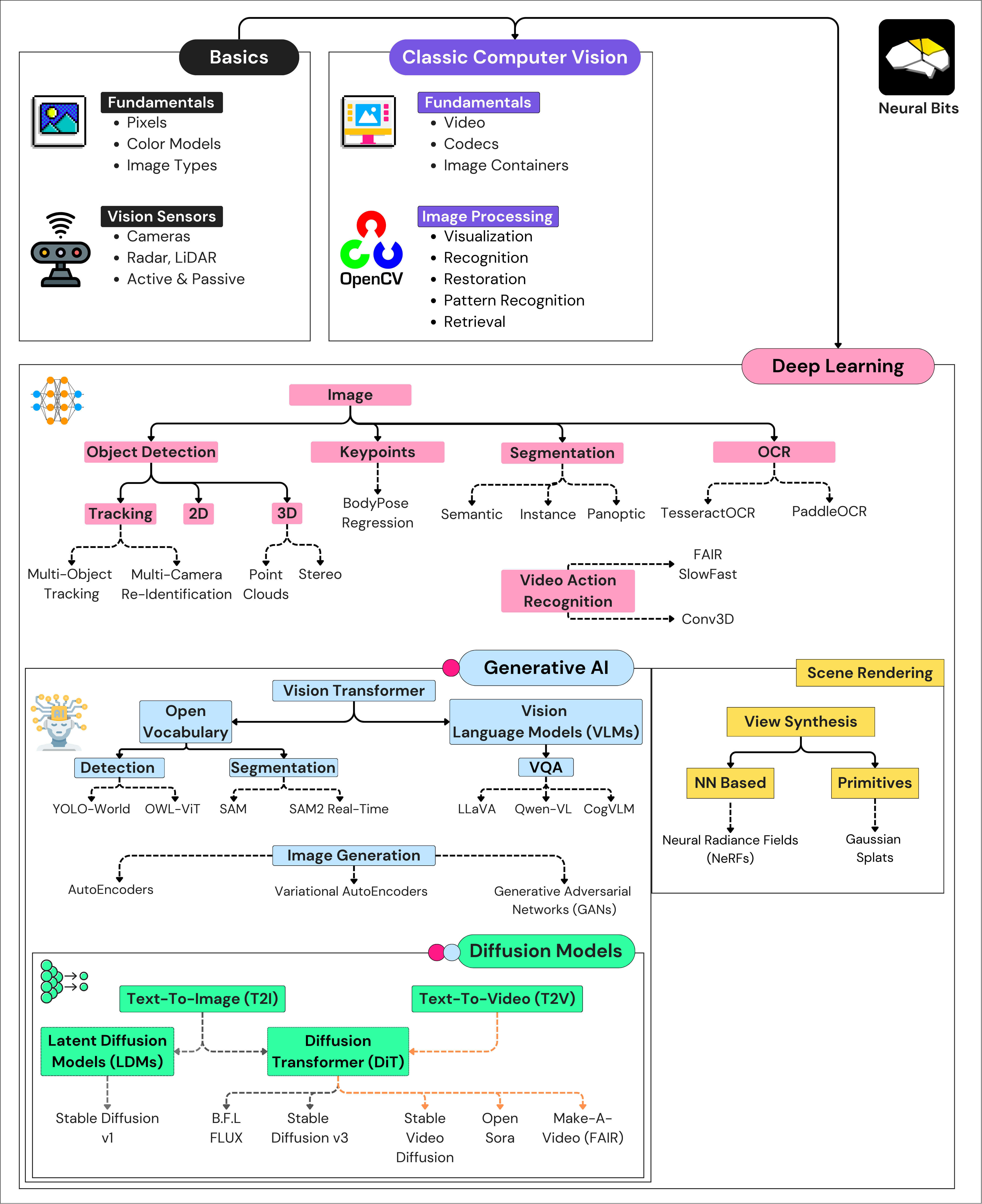
In this article, you’ll learn about:
Basics in Vision Sensors, Pixels, Color Modes, Images
Image and Video Processing with OpenCV
Object Detection in 2D and 3D, Single/Multi Camera Tracking
Semantic/Panoptic Image Segmentation
How Tesla’s Autopilot Vision System see the world
Photorealistic Scene Rendering with NERFs, Gaussian Splats
Generative AI in Computer Vision
AutoEncoders, GANs, Visual Transformer
Zero-Shot Object Detection, Segmentation
Open-Vocabulary Large Vision Models (LVMs)
Diffusion Models Explained
How T2I (text-to-image) works, Stable Diffusion, FLUX
How T2V (text-to-video) works, OpenAI Sora, Stable Video Diffusion (SVD)
This is a long article in which I aim to explain every key innovation in the Computer Vision field of AI, starting with the basics of digital pixels and sensors and moving on to Generative AI, large vision language models (LVLMs), and Text-to-Video Diffusion Transformers.
I recommend jumping directly to your topic of interest, where you’ll find visuals, explanations, and up-to-date references. The map below will help find everything discussed in this article.
What is Computer Vision?
Computer Vision is a subfield of Deep Learning that uses visual input, such as digital images and videos, to extract and derive meaningful information and allow systems to make decisions.
It’s one of the most mature applications of Machine Learning in the industry, with common examples being Autonomous Driving, Crowd Analysis, Manufacturing, Robotics, Retail, Augmented Reality, Art Generation, and many more.
References:
[1] Boesch, G. (2023, January 16). The 10 Best Computer Vision Books in 2024 - viso.ai. Viso.ai.
Sensors
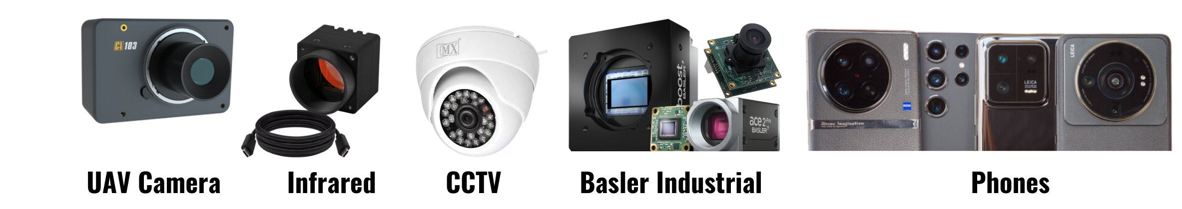
Devices for capturing visual data can be broadly split into Active and Passive categories.
Cameras on our Phones, Laptops, and Professional or Industrial cameras are passive sensors because they don’t emit any light into the environment but rather capture and record the existing reflected light when a picture is taken.
On the other hand, sensors such as LiDAR or Radar are active because they emit signals that propagate through the environment which are then captured and measured.
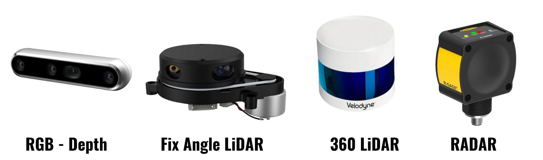
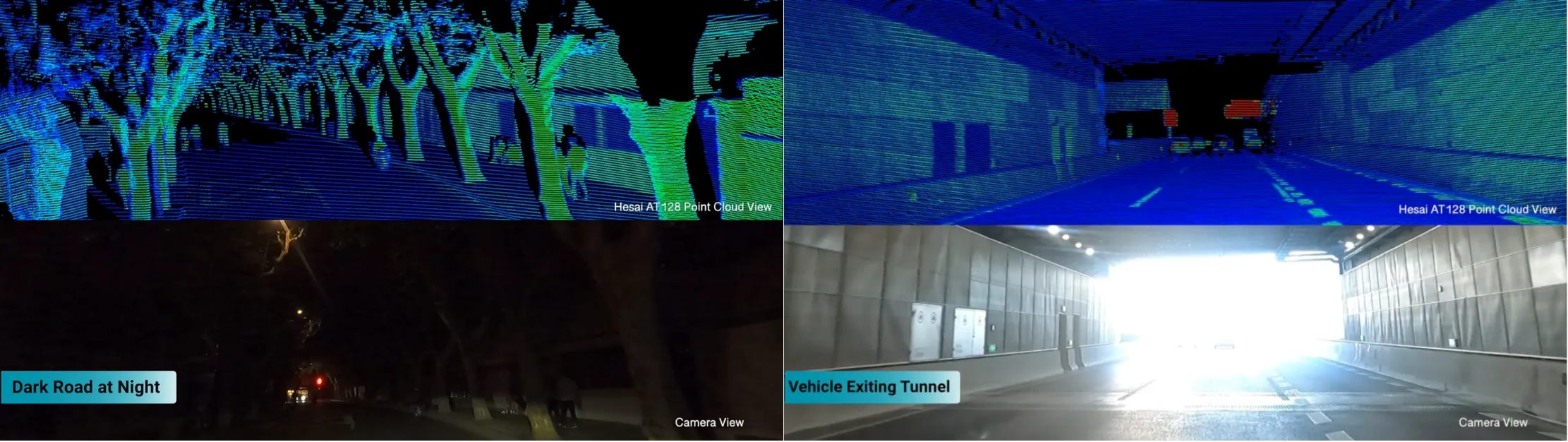
Due to signal emitting, the LiDAR sensor is used for deepwater scanning or underground mapping as they work in too bright/too dark environments whereas cameras work only when there’s the right amount of light in the scene.
Active sensors such as RGB-D cameras, LiDARs, or RADARs capture spatial information. This modality is key in developing applications requiring depth perception and understanding of 3D scenes in real-world environments. Features such as measuring real-world distance, sizes, and localization of objects in a 3D plane are made possible using spatial information. The most notable applications are AR (Augmented Reality), Game Development, Body Tracking, and Autonomous Driving.
Resources:
[1] Vina, A. (2024, 17 October). Computer vision cameras and their applications. Ultralytics.com
[2] McMinn, E. (2024). Understanding LiDAR: Technology and Applications. Flyability.com.
[3] FUJIFILM Exposure Center – USA. (2024, April 15). Camera sensors: What are they and how do they work?
Understanding Pixels, Colors, and Images
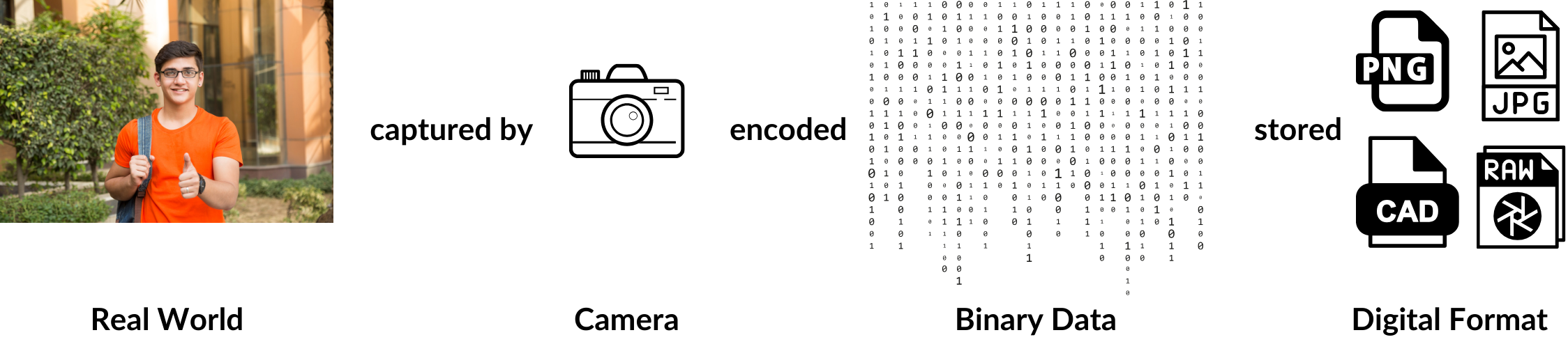
A pixel [3] (i.e. picture element) is the smallest unit in a digital image. Each pixel contains information about color or intensity at a specific location in the image. In most display devices, pixels are the smallest element that software can manipulate.
A color model is an abstract mathematical model that describes how colors can be represented as tuples of numbers. To define a digital image, we can distinguish between different color models, grouped into two categories:
Additive/Subtractive [1] - which contains the RYB (i.e red, yellow, blue), RGB (i.e red, green, blue), CMY (i.e. cyan, magenta, yellow), and CMYK (i.e. cyan, magenta, yellow, black) models.
Cylindrical [1] contains the HSL (i.e. hue, saturation, lightness), HSV (i.e. hue, saturation, value), and lesser-known Munsell and Natural Color System models.
In computer vision and image analysis, the additive RGB model dominates the color representation format, whereas cylindrical models are predominantly used within color pickers and image editing software.
When pixels encode positional and color information, they are arranged in a two-dimensional matrix (i.e., grid). This results in a digital image [4], also known as a raster image, where each pixel holds quantized values as integers that can be displayed on digital screens.
References:
[1] HSL and HSV - Wikipedia.(2022).Wikipedia.org
[2] Color Model - Wikipedia.(2002, December 19, ). Wikipedia.org
[3] Pixel - Wikipedia.(2001, October 30). Wikipedia.org
[4] Digital Image - Wikipedia. (2004, March 4). Wikipedia.org
Image Data Structures in Python
Before diving into how Images are represented programmatically, let’s identify the main differences between common image formats, used in multimedia.
To differentiate between types, we could split these into three categories: Rasterized, Vectorized, and Raw:
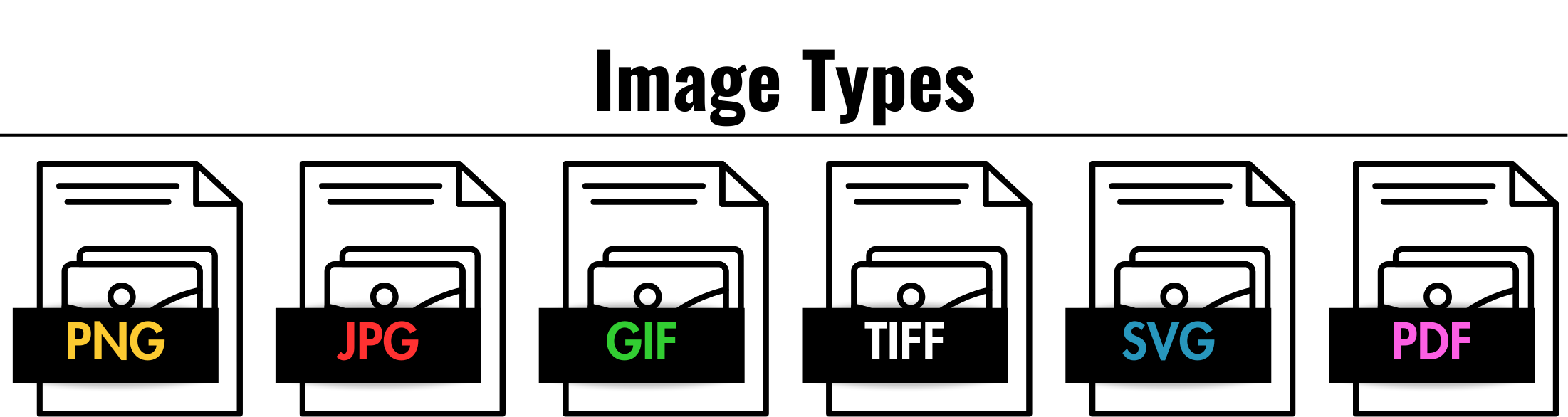
The term Rasterized image describes the format that stores image information as a grid of pixels in a 2D matrix, such as PNG, JPG, BMP, GIF, and TIFF.
Key details to remember:
JPG - lossy compression, smaller file size, web design/social media.
PNG - lossless compression, allows transparency channel and is higher in size.
BMP - uncompressed, high image quality.
TIFF is high quality, supports layers, and supports lossless compression.
GIF - limited to 256 colors, animated images.
WEBP - developed by Google to replace JPG, used mainly on the Web.
In Vectorized images, information is not bounded to the pixel level but rather described by mathematical equations, allowing elements to be upscaled/downscaled to any resolution without losing quality. Widely known formats are SVG and PDF.
Key details to remember:
SVG - infinitely scalable, small file size, editable in text.
PDF - can embed both raster and vector graphics, widely used.
The Raw format is used in professional photography where the image data is unprocessed or minimally processed. Formats strictly defined by the camera include HEIC (Apple Cameras), KDC (Kodac), RW2 (Panasonic), and SR2 (Sony).
Key details to remember:
HEIC - high quality, large file sizes, limited compatibility.
When working with images programmatically in Python, they are generally represented as rasterized images, a two-dimensional (2D) array of pixel values, where each pixel defines the intensity or color information for that point in the image. In Python, images are commonly stored using either: NumPy (via OpenCV) array container [1] which allows the manipulation of images at the lowest level (i.e. pixel level), and Pillow (PIL) container which abstracts the pixel level and offers higher-level functions.
With Numpy(OpenCV), images can be represented as:
Grayscale - single channel, (width, height)
Color (RGB/BGR) - 3 channels, (width, height, color_channels)
RGBA (PNG transparent) - 4 channels (width, height, color_channels, alpha) where alpha represents the transparency channel.
RGBD (depth images) - 4 channels (width, height, color_channels, grayscale_depth), apart from the standard color, we also have a grayscale channel with [0, 255] depth intensity for each pixel.
With PIL.Image [2] container, the image data storage container differs from NumPy, but the format interchange remains seamless:
RGB - 3 channels, RGB (width, height, color_channel) with each pixel taking 3 bytes of memory.
P (palettized) - 1 channel with each pixel taking 1 byte because it represents an index in a color palette with 256 colors.
L (grayscale)- 1 channel image, normally interpreted as grayscale.
References:
[1] Images are numpy arrays — Image analysis in Python. (2020). Scikit-Image.org.
[2] Image Module. (2025). Pillow (PIL Fork).
Getting started with OpenCV
OpenCV (Open Source Computer Vision Library) is a powerful, open-source CV (computer vision) and ML (machine learning) software library that provides a common infrastructure for CV applications. It contains over 2500 optimized algorithms for digital image processing, starting from basic functionality such as image resizing, changing colors, or applying color filters up to real-time video processing, motion detection, frame difference, frame similarity, and more.
When starting with Computer Vision or working on anything related to Image/Video processing in Python or C++, OpenCV is the developer’s choice.

Let’s overview a few key functionalities when working with Images using OpenCV:
Image Read, Display, and Save
## Read and Display Images ##
image = cv2.imread('image.png', cv2.IMREAD_COLOR)
cv2.imshow("Window", image)
cv2.waitKey(0)

## Save Image to Disk ##
cv2.imwrite("saved_image.png", image)
Video Player
## Display WebCam Video ##
cap = cv2.VideoCapture(0)
while True:
    ret, frame = cap.read()
    if not ret:
        break

    cv2.imshow('Video Stream', frame)
    if cv2.waitKey(1) & 0xFF == ord('q'):
        break

cap.release()
cv2.destroyAllWindows()
Manipulating Images
## Resizing ##
image = cv2.resize(image, (640, 640)) # to 640x640 resolution

# Flip X-axis
flipped_horizontally = cv2.flip(image, 1)

# Flip Y-axis
flipped_vertically = cv2.flip(image, 0)

# Flip XY axes
flipped_both = cv2.flip(image, -1)

## Colors ##
image = cv2.cvtColor(image, cv2.COLOR_BGR2RGB)  # from BGR to RGB
image = cv2.cvtColor(image, cv2.COLOR_BGR2GRAY) # grayscale
Cropping from an Image
x1,y1,x2,y2 = 50, 100, 400, 600
roi = image[x1:y1, x2:y2]
Drawing Objects
# Rectangle [img, x1y1, x2y2, color, thickness]
cv2.rectangle(image, (50, 50), (200,200), (255, 0, 0), 2)

# Circle [img, center, radius, color, thickness_fill)
cv2.circle(image, (150, 150), 50, (0, 255, 0), -1)

# Line [img, start, end, color, thickness]
cv2.line(image, (0, 0), (300, 300), (0, 0, 255), 3)  # Red line with thickness 3
Apart from the basic functionality described and showcased above, OpenCV also contains a large suite of optimized image processing techniques and filters.
Understanding Image Processing
Image processing refers to transforming an image into a digital form and performing certain operations to extract useful information from it. We can distinguish 5 main types of classical image processing:
Visualization - finding objects that are not visible in the image.
Recognition - identify or detect objects in the image.
Restoration - enhance the image from the original one.
Pattern Recognition - measure various patterns around the objects in the image.
Retrieval - search and retrieve similar images from a large database of images.
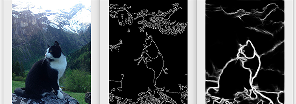
For visualization, we can use the Canny filter which picks hidden delimitations in the image by color differences at the pixel level, such as edges delimited by an intensity threshold.
Although not used directly in this format, edges in a picture or surrounding an object are important features learned by the convolution filters in a Convolutional Neural Network, and can be considered core triggers for Deep Learning tasks such as Image Classification, Segmentation, or Object Detection, more on these later.
import cv2

image = cv2.imread('image.jpg', cv2.IMREAD_GRAYSCALE)
edges = cv2.Canny(image, 50, 150) # color intensity threshold >50, <150

cv2.imshow('Edges', edges)
cv2.waitKey(0)
For Recognition [3], we can apply the CascadeClassifier, which uses a set of pre-defined features for objects and then scans the entire image for those features. In this example, I’m showcasing the use of a built-in frontal-face HAAR cascade to look up and detect faces in an image.
HAAR cascades could be considered a precursor to current Object Detection via Convolutional Neural Networks as they utilize a set of rectangular features (like edges and lines) to represent objects, in this case, the features of a face. Initially, the algorithm needs a lot of positive images (images of faces) and negative images (images without faces) to train the classifier. Then we need to extract features from it.

face_cascade = cv2.CascadeClassifier(cv2.data.haarcascades + 'haarcascade_frontalface_default.xml')

image = cv2.imread('face.jpg')
gray = cv2.cvtColor(image, cv2.COLOR_BGR2GRAY)

faces = face_cascade.detectMultiScale(gray, scaleFactor=1.1, minNeighbors=5)

for (x, y, w, h) in faces:
    cv2.rectangle(image, (x, y), (x+w, y+h), (255, 0, 0), 2)

cv2.imshow('Face Detection', image)
cv2.waitKey(0)
For Restoration [3], we could use the GaussianBlur function, to remove or smoothen the noise present in the image, giving us a sharper, enhanced image. It uses a Gaussian to determine how much to blur each pixel based on its distance from surrounding pixels, reducing noise and blending in the quality and appearance of a noisy image.

noisy_image = cv2.imread('image.jpg')

restored_image = cv2.GaussianBlur(noisy_image, (5, 5), 0)
cv2.imshow('Noise Reduction', restored_image)
cv2.waitKey(0)
For Pattern Recognition [3,4], we could use MatchTemplate, which takes an input image representing the template (e.g., an object crop) and slides it across another image, comparing blocks pixel by pixel to identify patterns of this object, left → right, up → down. If they match, the pixel coordinates of where the matched template region starts are saved in the output result.
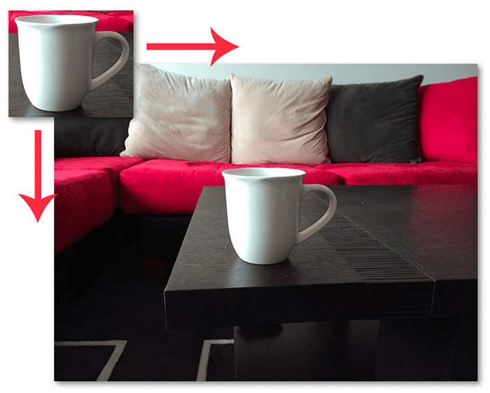
image = cv2.imread('image.jpg')
template = cv2.imread('template.jpg')

image_gray = cv2.cvtColor(image, cv2.COLOR_BGR2GRAY)
template_gray = cv2.cvtColor(template, cv2.COLOR_BGR2GRAY)

t_h, t_w = template_gray.shape

result = cv2.matchTemplate(image_gray, template_gray, cv2.TM_CCOEFF_NORMED)

min_val, max_val, min_loc, max_loc = cv2.minMaxLoc(result)

top_left = max_loc
bottom_right = (top_left[0] + template_width, top_left[1] + template_height)

cv2.rectangle(image, top_left, bottom_right, (0, 255, 0), 2)

cv2.imshow('Matched Template', image)
cv2.waitKey(0)
For Retrieval [5] OpenCV offers a suite of efficient algorithms including SURF (Speeded-Up Robust Features), SIFT (Scale-Invariant Feature Transform), and ORB (Oriented FAST and Rotated BRIEF). These algorithms identify distinctive features in images, making them optimal for image matching.
As these algorithms are an older approach that helped pioneer Computer Vision, let’s focus only on a few key details:
SURF - creates descriptors by analyzing the distribution of HAAR wavelets, which is faster than SIFT.
SIFT - detects a high amount of key points at different scales using differences of Gaussians and it’s computationally intensive, especially on larger images.
ORB - significantly faster than SIFT/SURF, making it suitable for real-time applications, but if the viewpoint of images changes it might be less robust compared to SIFT/SURF.
import cv2
import numpy as np

image = cv2.imread('image.jpg')
gray = cv2.cvtColor(image, cv2.COLOR_BGR2GRAY)

surf = cv2.SURF()

# Only features, whose hessian is larger than hessianThreshold are retained by the detector
surf.hessianThreshold = 500
keypoints, descriptors = surf.detectAndCompute(gray, None)

image = cv2.drawKeypoints(image, keypoints, flags=cv2.DRAW_MATCHES_FLAGS_DRAW_RICH_KEYPOINTS)

cv2.imshow('Feature Method - SURF', image)
cv2.waitKey()
cv2.destroyAllWindows()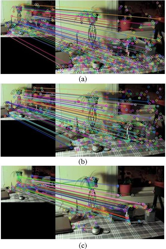
References:
[1] Alvi, F. (2024, December 5). Why you need to start learning OpenCV in 2025! OpenCV.
[2] OpenCV: Image processing in OpenCV. (n.d.).
[3] Koul, N. (2023, December 21). Image Processing using OpenCV — Python - Dr. Nimrita Koul - Medium. Medium.
[4] Ahedjneed. (2022, December 19). 15 image filters with Deployment|OpenCV|Streamlit.
[5] Karami, E., Prasad, S., & Shehata, M. (2017). Image matching using SIFT, SURF, BRIEF and ORB: Performance Comparison for distorted images.
Deep Learning Techniques
Being the go-to library for Computer Vision, OpenCV offers a large suite of Image Processing functionality, but by adding heuristics on top of heuristics, we cannot build a system that can generalize well. When applying any Image Processing filter, we obtain image features, which are pieces of information about an image's content. Usually, features might be specific structures in an image, such as points, edges, corners, contours, or objects.
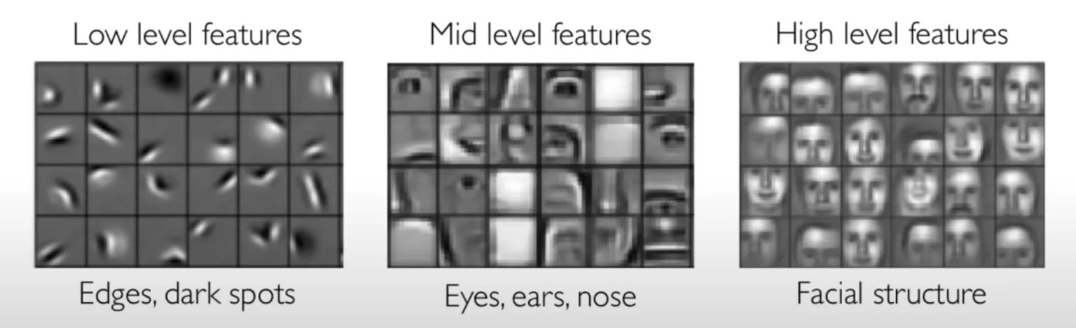
With CNNs (Convolutional Neural Networks) we stack multiple layer sets, such as Convolution + Pooling + Activation, that pick up various features from images, sometimes hidden and unachievable using standard filters - and then learn to generalize at a broader level.
The learnable features can be grouped into low-level and high-level based on the layer or region of the neural network where they are learned.
By training deep neural networks to process large volumes of images, the models can identify patterns that help in understanding a larger distribution of different patterns.
Computer Vision tasks, from basic Image Classification to complex 3D scene reconstruction address challenges in diverse fields like healthcare, robotics, autonomous driving, and entertainment. Below is an overview of the most important computer vision tasks and their applications.
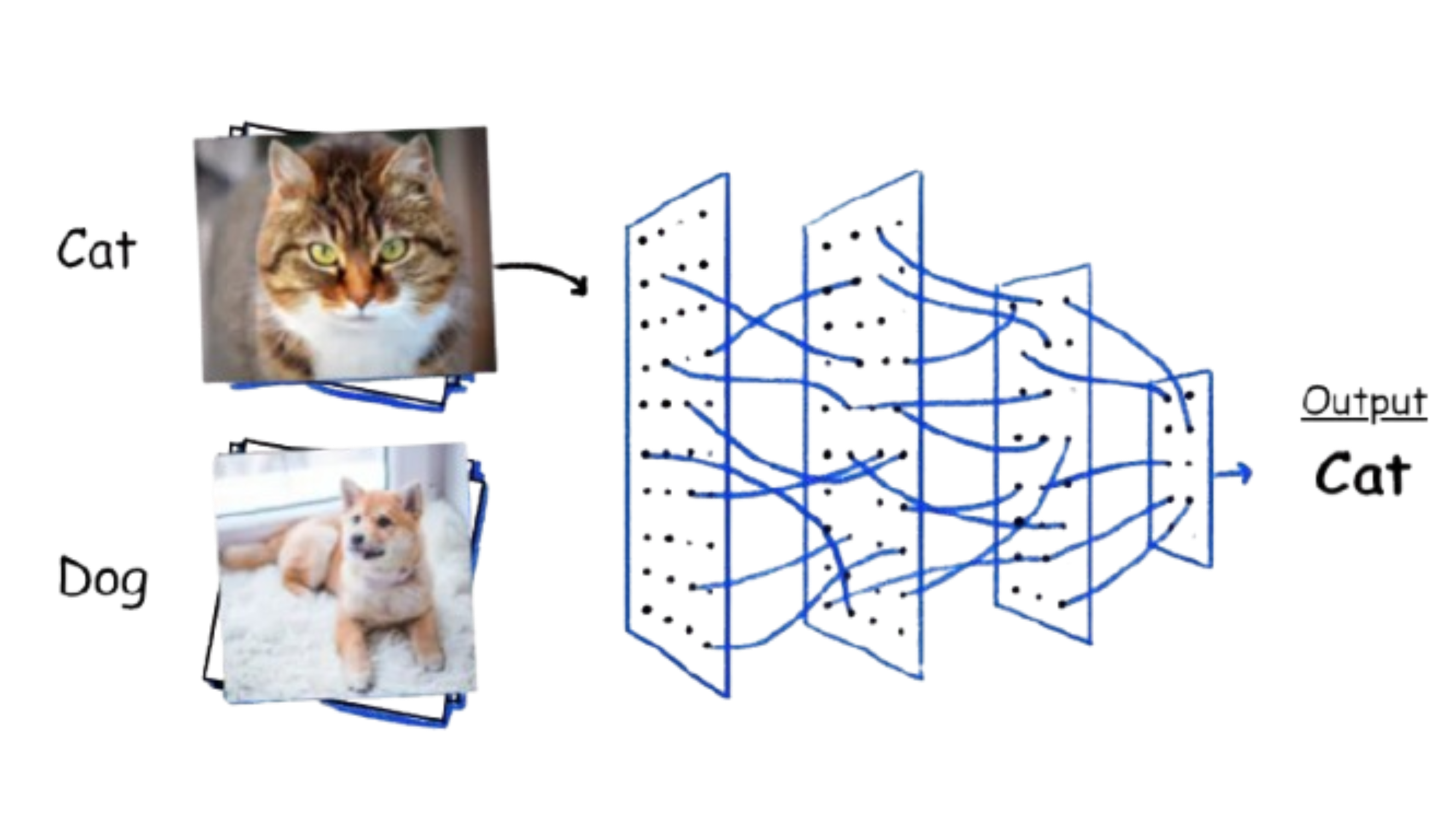
Image Classification
This task aims to classify the contents of an entire image to a specified label. The model takes an image as input and outputs a single value representing either a 0/1 (true/false) value for Binary Classification or the class ID for Multiclass Classification.
References:
[1] Convolutional Neural Networks & Computer Vision | KNIME. (n.d.). KNIME.
[2] Boesch, G. (2024, October 18). A complete guide to image classification in 2025. viso.ai.
[3] Papers with Code, (2025).Image Classification.
2D Object Detection
For 2D Object Detection, we want to identify objects in an image by localizing them with bounding boxes and classifying them with labels. Object Detection acts at an object level, meaning it focuses on detecting individual objects within an image and understanding their positions and categories.
We can summarize Object Detection into 2 tasks:
Localization:
Identifying the precise location of an object within the image.
Represented by bounding boxes, defined by their top-left corner coordinates (x_min, y_min) and their width and height (w, h).
Classification:
Assigning a class label to each detected object (e.g. car, dog, person).
The model outputs probabilities for each possible class, and the label with the highest confidence is chosen.
As an image is passed through a CNN (Convolutional Neural Network), the earlier layers of the network extract low-level features like edges, textures, and corners, while the deeper layers focus on high-level, semantic features that represent parts or entire objects.
Toward the deeper layers, the network generates higher-level feature maps highlighting regions with high activation values, indicating where the network has detected features corresponding to objects. For each cell in a feature map, the network head learns to regress the bounding box coordinates, yielding multiple bounding-box proposals for each object.
Further, a post-processing stage such as NMS [7] (Non-Maximum Suppression) is commonly applied to reduce the detection to a single bounding box by collapsing smaller and encapsulated bounding boxes into a single, bigger one.
References:
[1] YOLOv8 Object Detection Model: What is, How to Use. (n.d.).
[2] Grounding DINO. (n.d.).
[3] facebookresearch/detectron2: Detectron2 is a platform for object detection, segmentation and other visual recognition tasks. (n.d.). GitHub.
[4] Papers with Code - 2D Object Detection. (n.d.).
[5] Agarwal, R. (2019, April 30). Object Detection: an end to end theoretical perspective. Medium.
[6] Chen, W., Li, Y., Tian, Z., & Zhang, F. (2023). 2D and 3D object detection algorithms from images: A Survey. Array, 19, 100305.
[7] A Deep Dive Into Non-Maximum Suppression (NMS) | Built In. (2023). Built In.
Object Tracking
Building on initial object detections by assigning a unique identifier to each detected object, Object Tracking ensures that objects are continuously monitored as they move across frames, maintaining their identities over time. A key advantage of object tracking is its ability to compensate for inconsistencies in object detection, saving both performance and cost.
For example, if an object is successfully detected in Frame #1 of a video, but is missed in frames #2, #3, and #4 - the tracking component will maintain the object's trajectory and identity. To do that, it can either use a single estimation algorithm such as the Kalman Filter to predict the object state (i.e position, velocity, acceleration) with heuristics only (i.e bounding box position) or use a combination of descriptors such as Kalman + CNN encoders for better differentiation between objects.
This ensures smoother monitoring of dynamic or complex scenes.
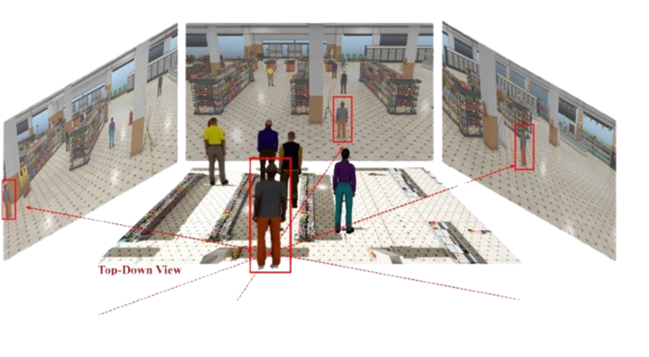
Object Tracking is mainly split into two scenarios, single camera tracking and multi-camera tracking and re-identification:
Single-Camera Tracking: Monitoring objects within a single video stream.

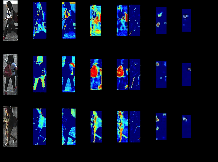
Multi-Camera Tracking with Re-Identification (ReID): Tracking objects across multiple cameras, where ReID techniques ensure that the same object is recognized even when it appears in different views or cameras.

A common ReID technique involves maintaining a centralized in-memory embedding database, which is fast and lightweight, such as FAISS or Redis.
Let’s understand the basic workflow:
A CNN is used to encode image crops of detected objects, from all cameras in the system.
An embedding vector for each object is then added to the in-memory Vector Database and kept as a short history.
When assigning unique object IDs, the system compares embedding vectors on a many-to-many relationship, retrieves the Top-K closest entries based on a similarity metric, and assigns the same ID across cameras.
References:
[1] Shin, P. (2023, April 20). State-of-the-Art Real-time Multi-Object Trackers with NVIDIA DeepStream SDK 6.2 | NVIDIA Technical Blog. NVIDIA Technical Blog.
[2] Dipert, B. (2024, August 2). Enhance Multi-camera Tracking Accuracy by Fine-tuning AI Models with Synthetic Data. Edge AI and Vision Alliance.
[3] Klingler, N. (2024, June 21). Object Tracking in Computer Vision (2024 Guide). viso.ai.
[4] Papers with Code - Object Tracking. (n.d.).
[5] Jegou, H., Douze, M., & Johnson, J. (2018, June 28). Faiss: A library for efficient similarity search. Engineering at Meta.
Image Segmentation
Image segmentation is a computer vision technique that partitions a digital image into discrete groups of pixels—image segments—to inform object detection and related tasks.
On Image Segmentation, we have 3 subcategories:
Semantic Segmentation - each pixel has its class
Instance Segmentation - differentiate instances
Panoptic Segmentation - combines both, Instance and Semantic.
Semantic Segmentation [1], groups each pixel in an image to a single category class. In the picture below, for example, the water area is sea class, and all objects are mammal class.

For Instance Segmentation [2], we extend semantic segmentation by distinguishing individual instances of the same class. In the example below, the mammal class from Semantic Segmentation is now split into different class instances, Human and Dog.

For Panoptic Segmentation [3], we unify the Semantic and Instance segmentation into one task. It assigns a unique ID to every pixel to delimit individual instances and semantic regions, enabling a more detailed understanding of a given scene.

References:
[1] Image segmentation detailed overview [Updated 2024] | SuperAnnotate. (n.d.). SuperAnnotate.
[2] Semantic segmentation: Complete guide [Updated 2024] | SuperAnnotate. (n.d.). SuperAnnotate.
[3] Bonnet, A. (2024, November 6). Guide to Panoptic Segmentation.
[4] Papers with Code - Image Segmentation. (n.d.).
[5] Top Instance Segmentation Models Models. (2023). Roboflow.com.
3D Object Detection
Is the task of identifying and localizing objects in a 3D space using spatial information from sensors like LiDAR, depth cameras, or stereo vision. Unlike 2D detection, which uses bounding boxes in a single image plane, 3D object detection provides information about an object’s XYZ position, size, and orientation in real-world coordinates.
Detecting objects in 3D scenes is crucial for Autonomous Driving, AR (Augmented Reality), and Robotics as without scene perception these systems cannot operate in the real world.
For models to learn real-world spatial information about objects, a multimodal input is required, combining data from images and point clouds or depth sensors. In robotics and autonomous driving, this concept is referred to as “Sensor Fusion”, which refers to merging Image information and Spatial information into the same data pool. Currently, the LiDAR sensor offers the densest 3D scans of objects, where each pixel is mapped to a point in space obtaining a “Point Cloud”.
A PointCloud is a 3D data structure composed of points, each defined by XYZ coordinates in a 3D space, with the Z axis commonly indicating the absolute distance to the scanned object.
As an active sensor, LiDAR usually contains a rotating laser arm which emits laser beams into the environment and when these rays strike a surface, they bounce back and are captured, registering the information, resulting in an accurate 3D representation of the environment.

The default PointCloud doesn’t contain color, but rather a depth map representation (i.e light-gray points are closer, dark gray points are farther), on top of which we can add the color image modality to map color texture to the 3D pixel from the depth map.
See the example below, where brighter colors indicate closer distance.

References:
[1] google-ai-edge/mediapipe: Cross-platform, customizable ML solutions for live and streaming media. (n.d.). GitHub.
[2] Getting started - Open3D 0.18.0 documentation. (n.d.).
[3] Papers with Code - 3D Object Detection. (n.d.).
[4] TianhaoFu/Awesome-3D-Object-Detection: Papers, code and datasets about deep learning for 3D Object Detection. (n.d.). GitHub.
[5] open-mmlab/mmdetection3d: OpenMMLab’s next-generation platform for general 3D object detection. (n.d.). GitHub.
[6] open-mmlab/OpenPCDet: OpenPCDet Toolbox for LiDAR-based 3D Object Detection. (n.d.). GitHub.
[7] Hackster.io. (2022, April 19). Point-Clouds based 3D-Object-Detection on PYNQ-DPU. Hackster.io; Hackster.
[8] The KITTI Vision Benchmark Suite. (2015). Cvlibs.net.
Keypoints Detection
With keypoint detection, we aim to identify the location of an object which requires a more detailed delimitation than a bounding box, such as a polygon. The most common applications are BodyPose [1] estimation used to identify Body Segments (e.g. fingers, arms, legs) or Face Landmarks used for FaceID or in A/R (Augmented Reality) filters such as Snapchat or Instagram face filters.
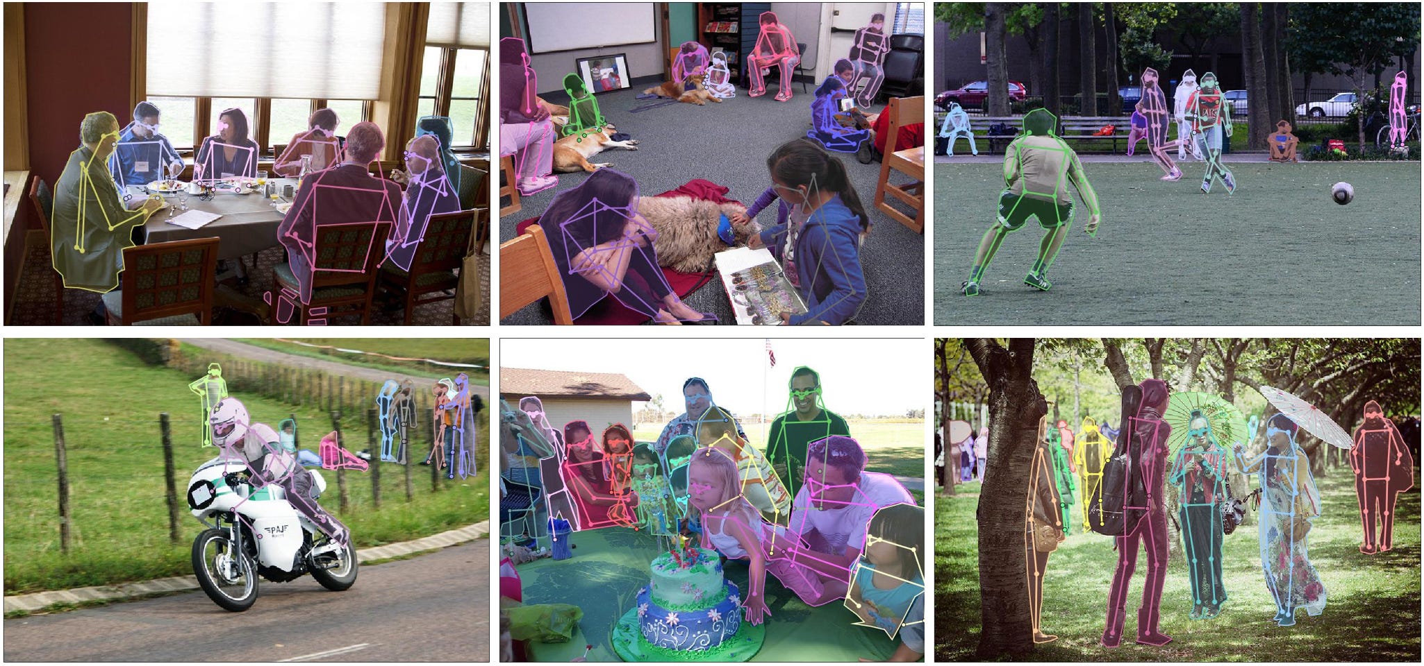
When training a points detection model, the approach is similar to Object Detection, as instead of localizing objects with a bounding box and classifying them with a label ID, we classify each key point using a label ID.
A common application for BodyPose detection is the Personal Gym Trainer app, allowing users to improve exercise form and rhythm.
References:
[1] Odemakinde, E. (2023, October 4). Human Pose Estimation - Ultimate Overview in 2025 - viso.ai. Viso.ai.
[2] 3D Pose Detection with MediaPipe BlazePose GHUM and TensorFlow.js. (2021). Tensorflow.org.
Complex CV Systems in the Real World
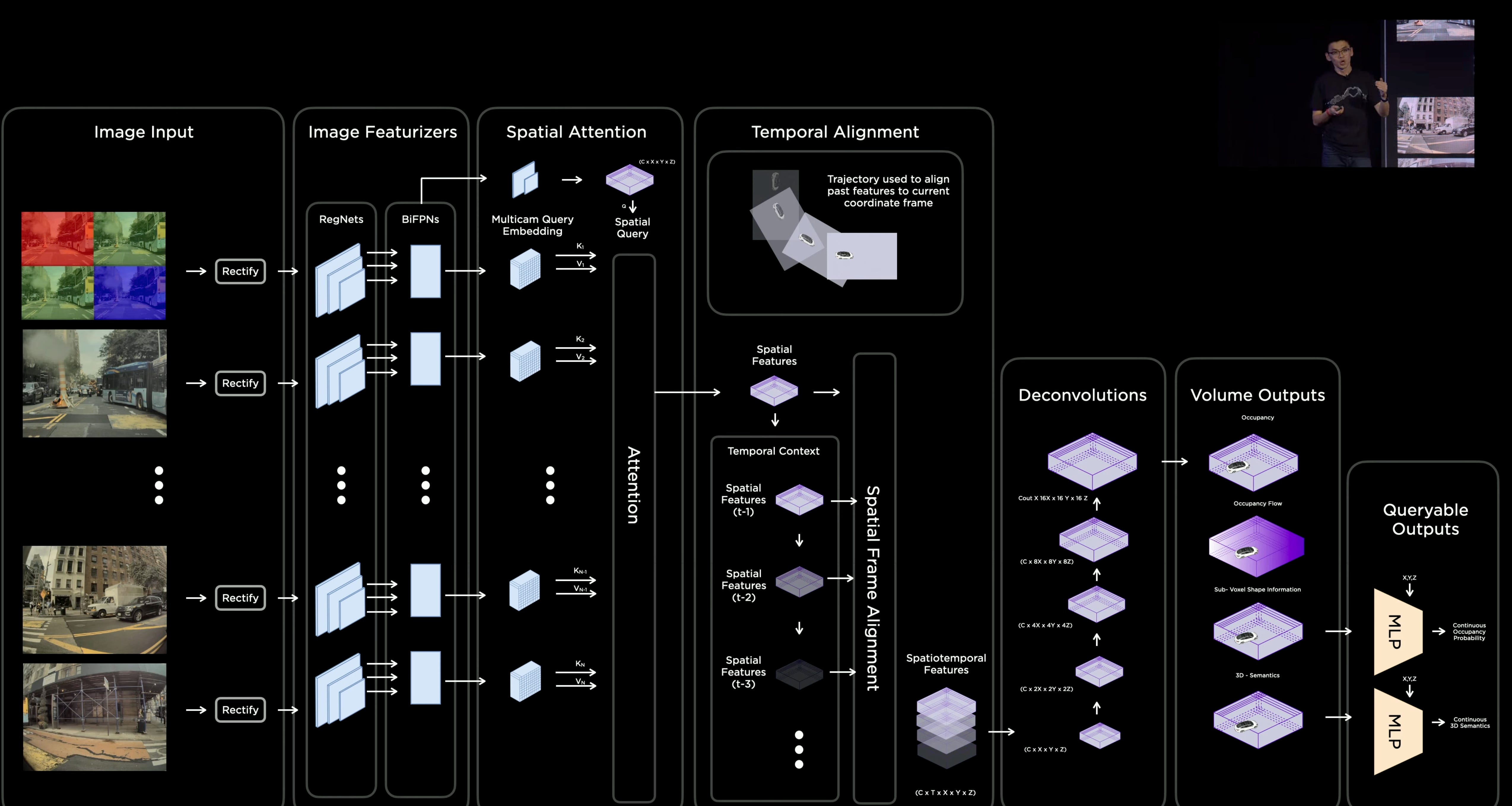
One of the most complex Computer Vision systems is the Tesla Autopilot, which uses a multi-camera setup around the car and employs tasks such as 2D & 3D Object Detection, Panoptic Segmentation, Object Tracking, 3D environment mapping, drive lane prediction, and many more.
The default approach to self-driving used a sensor-fusion mechanism where Cameras, Lidar, and Radar sensors were giving a 3D mapping of the environment due to the inability of a camera-only system to output accurate real-world distances and 3D coordinates.
However, since 2021, Tesla started transitioning to a full camera-only vision system called Tesla Vision which processes the video inputs through an Occupancy Network that runs on in-car FSD chips and which outputs both 2D and 3D information.
Another self-driving solution is Waymo (previously known as Google Self-Driving Car), which still uses Lidars as its core sensor suite.

An OpenSource version for a driving assistant, which is vision-based on cameras, is proposed by George Hotz (a.k.a geohot) CEO of CommaAI, called OpenPilot with full code available on GitHub.

References:
[1] This is how Tesla’s Autopilot sees the world. (2020, February 3). WhichCar.
[2] Autopilot and Full Self-Driving Capability | Tesla Support United Kingdom. (2025). Tesla.
[3] commaai/openpilot: openpilot is an operating system for robotics. Currently, it upgrades the driver assistance system on 275+ supported cars. (2024, June 14). GitHub.
[4] Zhang, J. (2021, October 19). Deep Understanding Tesla FSD Part 2: Vector Space | Medium. Medium.
Video Action Recognition
The use cases and computer vision applications described above work on the spatial dimension of the vision channel. Detecting Objects or Segmenting portions of the image relies on a single time-point input, static image, or single frame from a video. Only object tracking acts as a heuristic to propagate information through the time channel, as it keeps the same ID for detected objects across time.
However, none of the models in these tasks use video directly as an input to the network.
Adding the temporal dimension enables models to take videos or sequences as input and analyze motion, activity, and dynamic events over time. One common use case is Action Recognition, where a model is fed a short video sequence and tries to predict the noticed behavior or action.

These models are often based on Conv3D layers, which process a block of pixels, in both the XY (space) dimension across an image and the T (time) dimension across a stack of images, successfully identifying both visual and temporal patterns.
References:
[1] facebookresearch/SlowFast: PySlowFast: video understanding codebase from FAIR for reproducing state-of-the-art video models. (2025). GitHub.
[2] Action Recognition. (2019). Computervision-Recipes.
Generative AI
Generative AI is a new emerging trend in Language Modelling and Computer Vision which refers to a class of deep learning algorithms capable of producing new data that resembles existing datasets. The generative AI algorithms are commonly based on the Transformer Neural Network Architecture.
Before diving in, let’s understand a few key terms:
Foundation Model - a deep learning model that is trained on vast datasets so it can be applied across a wide range of use cases, usually referred to as “downstream tasks”.
Token - chunks/parts of input data represented as D-dimensional vectors.
Tokenization - the process of transforming raw input data into appropriate tokens, with each modality (i.e. text, image, audio) following a different pattern. For example, for text - byte-pair-encoding is used, for image - non-overlapping image patches, and for audio-spectrogram patches as a 2D image.
Positional Encoding - a fixed-size vector representation of the relative positions of tokens within a sequence, it provides the transformer model with information about where the tokens are in the input sequence.
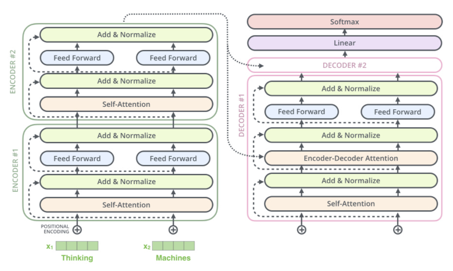
The raw input (i.e. text sentence for Language Modelling, image patch for Vision) is tokenized (i.e. split into tokens), then a positional embedding vector is added to each token, and only after that, is the input fed to the Transformer network.
As we’re focusing on the Vision modality, let’s cover the Vision Transformer.
Vision Transformer
A Vision Transformer is a neural network architecture for processing images, inspired by the transformers used in NLP. Unlike traditional convolutional neural networks (or CNNs), it uses self-attention mechanisms to analyze relationships between image parts.
First, the image is split into patches, and then the positional embedding vector for each patch is added such that we keep the structure of the image patches.
As the input passes through the transformer encoder layers, the model captures spatial and semantic interactions between patches providing a global representation of the image and learning hierarchical visual features.
This approach opens up new perspectives in object recognition, image segmentation, and other Computer Vision tasks.
 | by Ankit kumar | Medium")
Apart from Image Classification, the Vision Transformer also excels in Zero-Shot Image Segmentation, Zero-Shot Object Detection, Vision Question Answering (VQA), and more.
References:
[1] The Vision Transformer architecture: (2022). ResearchGate.
[2] Zhou, H., Zhang, R., Lai, P., Guo, C., Wang, Y., Sun, Z., & Li, J. (2024). EL-VIT: Probing Vision Transformer with Interactive Visualization. ArXiv.org.
[3] Dosovitskiy, A., Beyer, L., Kolesnikov, A., Weissenborn, D., Zhai, X., Unterthiner, T., Dehghani, M., Minderer, M., Heigold, G., Gelly, S., Uszkoreit, J., & Houlsby, N. (2020). An Image is Worth 16x16 Words: Transformers for Image Recognition at Scale. ArXiv.org.
Segment Anything, SAM, Facebook AI Research (FAIR)
The SAM (i.e. Segment Anything) [1] model from FAIR is the new SOTA foundation model for zero-shot instance segmentation tasks in Computer Vision. Trained on an immense dataset of 11M images and over 1B segmentation masks, it can segment any object in an image, without necessarily requiring fine-tuning for downstream task adaptation.
The segmentation model is part of the data flywheel which allowed FAIR to train, collect, and auto-annotate the biggest segmentation dataset to date, SA-1B which can be downloaded alongside SAM model checkpoints.
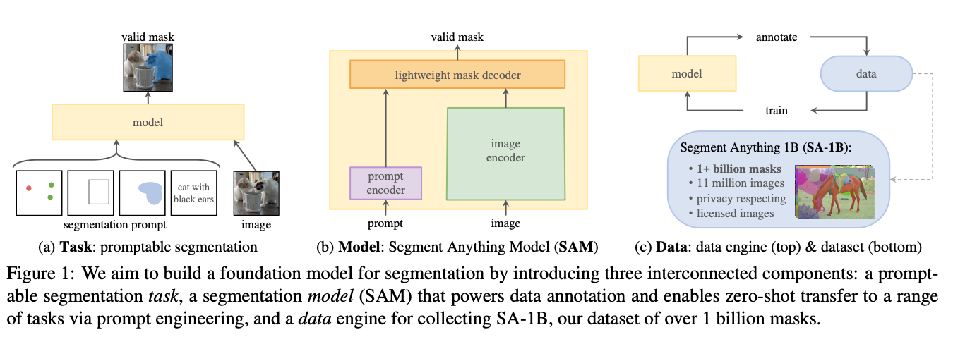
The next installment in the SAM model series is SAM 2 [2,3] - the first unified model for real-time, promptable object segmentation in images and videos, enabling a step-change in the video segmentation experience and seamless use across image and video applications.

References:
[1] Buhl, N. (2023, April 6). Meta AI’s Segment Anything Model (SAM) Explained: The Ultimate Guide. Encord.com; Encord Blog.
[2] Segment Anything. (2025). Segment-Anything.com.
[3] Meta Segment Anything Model 2. (2022). Meta.com.
Large Vision Language Models (LVLMs)
Vision language models can learn simultaneously from images and texts to tackle many tasks, from visual question answering (VQA) to image captioning.
VLMs [1] stand out for their ability to understand and synthesize information from both visual and textual data, offering a broader range of applications that require multimodal understanding. Using the Vision Arena leaderboard, let’s cover 3 popular architectures: LLaVA, Qwen-VL, and CogVLM.
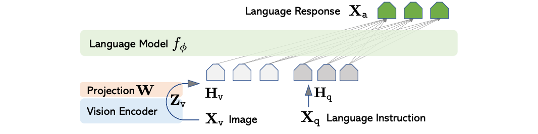
LLaVA
LLaVA [5] is an end-to-end trained large multimodal model that combines a vision encoder and Vicuna for general-purpose visual and language understanding. Comes in a 13B parameter size variant by default, parameters that are split across a Language Model, Vision Encoder, and an embedding projection layer between the two.
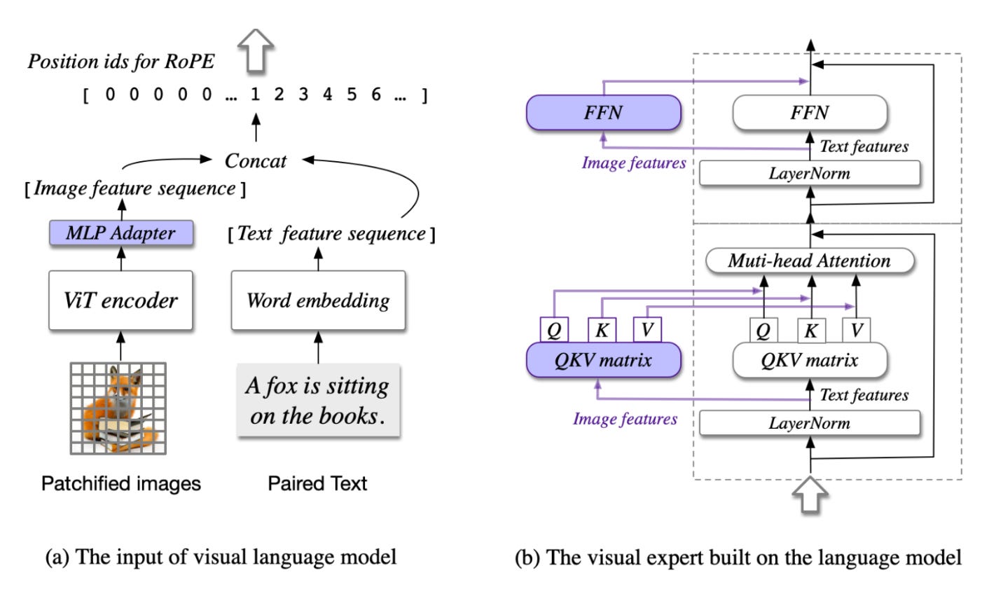
CogVLM
CogVLM [7] is a powerful open-source visual language model (VLM), with 17B model parameters, 10 billion for the vision model, and 7 billion for the language model. Different from the popular shallow alignment method which maps image features into the input space of the language model, CogVLM bridges the gap between the frozen pre-trained language model and image encoder by a trainable visual expert module in the attention and FFN layers.
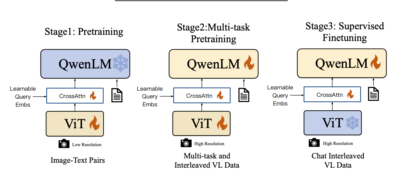
The Qwen-VL [4, 8] series is a set of large-scale vision-language models (LVLMs) designed to perceive and understand both texts and images. Developed by the Alibaba Group, it has a 9.6B parameter size, a 1.9B Vision Encoder, a 0.08B Vision-Language Adapter, and a 7.7 B large language model. It’s one of the few models that supports accurate multilingual text, including most European languages, Japanese, Korean, Arabic, Vietnamese, and Chinese.
References:
[1] Frederik Hvilshøj. (2023, April 24). Visual Foundation Models (VFMs) Explained. Encord.com; Encord Blog.
[2] Vision Arena (Testing VLMs side-by-side) - a Hugging Face Space by WildVision. (2025). Huggingface.co.
[3] Bai, J., Bai, S., Yang, S., Wang, S., Tan, S., Wang, P., Lin, J., Zhou, C., & Zhou, J. (2023). Qwen-VL: A Versatile Vision-Language Model for Understanding, Localization, Text Reading, and Beyond. ArXiv.org.
[4] Wang, P., Bai, S., Tan, S., Wang, S., Fan, Z., Bai, J., Chen, K., Liu, X., Wang, J., Ge, W., Fan, Y., Dang, K., Du, M., Ren, X., Men, R., Liu, D., Zhou, C., Zhou, J., & Lin, J. (2024). Qwen2-VL: Enhancing Vision-Language Model’s Perception of the World at Any Resolution. ArXiv.org.
[5] haotian-liu/LLaVA: [NeurIPS’23 Oral] Visual Instruction Tuning (LLaVA) built towards GPT-4V level capabilities and beyond. (2024, January 31). GitHub.
[6] Vicuna: An Open-Source Chatbot Impressing GPT-4 with 90%* ChatGPT Quality | LMSYS Org. (2023). Lmsys.org.
[7] Zhang, Q. (2023, November 10). CogVLM Visual Expert for Pretrained Language Models. Qiang Zhang.
[8] QwenLM/Qwen2-VL: Qwen2-VL is the multimodal large language model series developed by Qwen team, Alibaba Cloud. (2025). GitHub.
Zero-Shot Object Detection
Traditionally, models used for object detection require labeled image datasets for training and are limited to detecting the set of classes from the training data. The surge of Vision Transformers allowed for models to leverage multi-modal representations to perform open-vocabulary detection.
Some powerful proprietary models with vision capabilities are OpenAI GPT4-V, xAi Groq2, Google Gemini, and others, but let’s focus on the open-source ones.
One of the oldest installments in using transformers for object detection is DETR (i.e. Detection Transformer) from Facebook AI Research (FAIR).

Newer models are YOLO-World and OWL-ViT.
YOLO-World builds on top of Ultralytics YOLO-v8 Object Detection model and adds a Vision-Language module to enable open-vocabulary detection.
Open-vocabulary detection (OVD) aims to generalize beyond the limited number of base classes labeled during the training phase. The goal is to detect novel classes defined by an unbounded (open) vocabulary at inference.

OWL-ViT combines CLIP embeddings with lightweight object classification and localization heads. The authors of OWL-ViT first trained CLIP from scratch and then fine-tuned OWL-ViT end to end on standard object detection datasets using a bipartite matching loss.
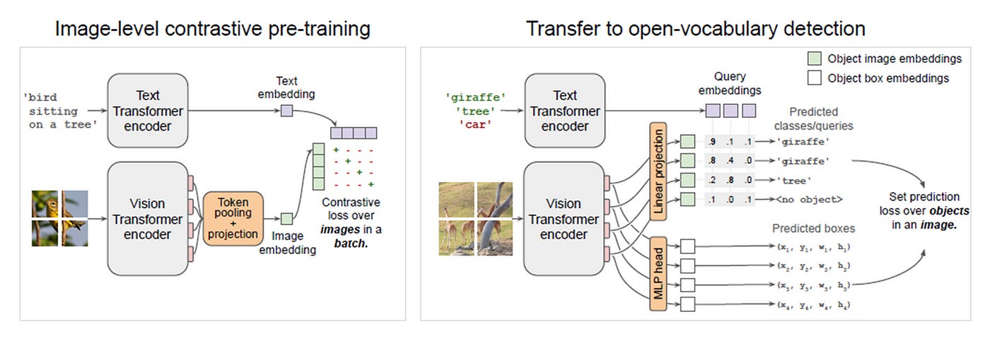
References:
[1] facebookresearch/detr: End-to-End Object Detection with Transformers. (2020, June 29). GitHub.
[2] OWL-ViT. (2017). Huggingface.co.
[3] Minderer, M., Gritsenko, A., Stone, A., Neumann, M., Weissenborn, D., Dosovitskiy, A., Mahendran, A., Arnab, A., Dehghani, M., Shen, Z., Wang, X., Zhai, X., Kipf, T., & Houlsby, N. (2022). Simple Open-Vocabulary Object Detection with Vision Transformers. ArXiv.org.
[4] AILab-CVC/YOLO-World: [CVPR 2024] Real-Time Open-Vocabulary Object Detection. (2024). GitHub.
[5] Cheng, T., Song, L., Ge, Y., Liu, W., Wang, X., & Shan, Y. (2024). YOLO-World: Real-Time Open-Vocabulary Object Detection. ArXiv.org.
Image Generation Models
Generative models learn patterns and distributions to synthesize new outputs, which include generating Images, Videos, 3D models, entire scenes, and more.

The progress of the current models such as StableDiffusion, DALL-E, and Midjourney build upon foundational architectures and concepts of Variational AutoEncoders(VAE) and GANs (Generative Adversarial Networks).
Let’s unpack this progression, in the following order: AE, VAE & GANs.
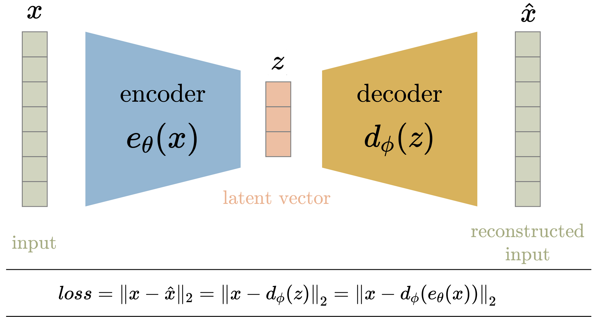
AutoEncoders (AE)
It is a neural network architecture designed to compress data into a lower-dimensional representation and reconstruct it back to its original form. The architecture consists of an Encoder that compresses input data into a latent representation and a Decoder that reconstructs data back to its original form.
The key point of AE’s is that they are deterministic, meaning that compression and reconstruction will always be the same.
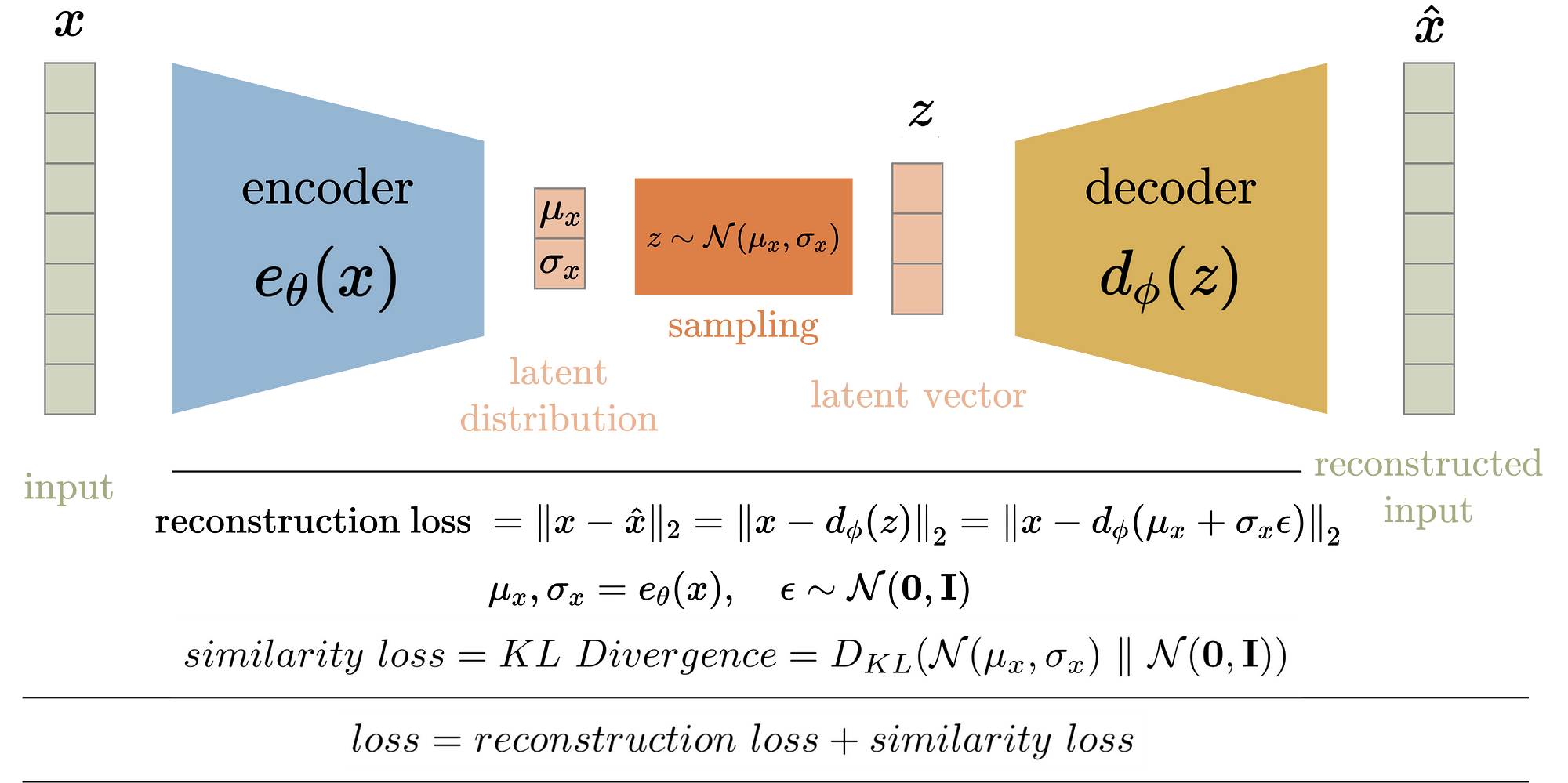
Variational Autoencoders (VAE)
A probabilistic extension of the autoencoder. It encodes data into a latent space and allows for generative sampling from this space. Compared to traditional autoencoders, VAEs [3] are not only designed for compression but also for generating new data.
GANs (Generative Adversarial Network)
A deep learning model architecture for generative modeling, where the goal is to create new data samples that resemble a given dataset, applicable to fields like image generation, video synthesis, and data augmentation.
The architecture consists of two neural networks, Generator and Discriminator, that play “a zero-sum game”, where:
The generator creates new data samples from random noise, and its goal is to produce samples indistinguishable from real data. It aims to fool the discriminator.
The discriminator evaluates whether a given sample is real (from the dataset) or fake (from the generator), aiming to classify correctly the real/fake samples. It aims to control the generator.
Further progression of GANs include:
Conditional GANs - using specific inputs such as labels, and images to control the generated output.
Cycle GAN - translating image from one domain to another without paired data samples (e.g. turning an image into a painting)
Style GAN - generates highly realistic images by controlling style at multiple levels of the generation workflow.
References:
[1] Boesch, G. (2024, October). Guide to Generative Adversarial Networks (GANs) in 2025 - viso.ai. Viso.ai.
[2] Variational Autoencoders. (2018, February 25). Variational Autoencoders. YouTube.
[3] Anwar, A. (2021, November 3). Difference between AutoEncoder (AE) and Variational AutoEncoder (VAE). Medium; Towards Data Science.
Diffusion Models
Building on previous concepts from VAE and GANs, Diffusion Models [2,3] generate data by gradual denoising a sample from random noise. They reverse a forward process of adding noise to data over several time steps, learning how to "undo" the noise and recover the original data distribution.
After training, we can use the Diffusion Model to generate new data by passing randomly sampled Gaussian noise through the learned denoising process.
The workflow of the diffusion process can be summarized in 4 steps:
Forward Diffusion
The image is progressively “corrupted” by adding Gaussian noise in a series of timesteps.

The forward diffusion step, animated [Source]
Reverse Diffusion Process:
A neural network, often a U-Net, is trained to predict and remove noise at each timestep, effectively denoising the data in reverse.
The reverse diffusion (noise removal) step, animated [Source]
Training Objective:
The model is optimized to minimize a variational lower bound (VLB) and it learns to estimate the noise or the data gradient at different noise levels.
Sampling:
Starting from random noise, the reverse process iteratively refines it, using the learned model, to generate coherent data samples.

One drawback of Diffusion Models is that they’re unconditional. Even if they can generate realistic images, they lack control. Users can’t specify what the model should generate beyond broad data properties.
To overcome this gap, diffusion models can be augmented with a text encoder to control the image generation workflow. Instead of a generic “dog” description for image generation, we can use “a golden retriever sitting on a white porch,” which is a guided generation. This transforms the task of random image generation into a guided text-to-image model.
References:
[1] O’Connor, R. (2022, May 12). Introduction to Diffusion Models for Machine Learning. News, Tutorials, AI Research.
[2] Ho, J., Jain, A., & Abbeel, P. (2020). Denoising Diffusion Probabilistic Models.
[3] Introduction to Diffusion Models for Machine Learning | SuperAnnotate. (2020). SuperAnnotate.
[4] Understanding Diffusion Models: An Essential Guide for AEC Professionals | NVIDIA Technical Blog. (2024, July 10). NVIDIA Technical Blog.
[5] Rethinking How to Train Diffusion Models | NVIDIA Technical Blog. (2024, March 21). NVIDIA Technical Blog.
[6] Lou, A. (2023). Reflected Diffusion Models | Aaron Lou. Aaronlou.com.
[7] Generative AI Research Spotlight: Demystifying Diffusion-Based Models | NVIDIA Technical Blog. (2023, December 14). NVIDIA Technical Blog.
Text Encoders
To capture the complexity and compositionality of arbitrary language text inputs, we need powerful semantic text encoders. In combination with Image Generation, text embeddings [4] help guide the process starting in a more refined local minimum in the latent space, allowing the image to be highly correlated with the text semantics of the input prompt description.
OpenAI CLIP
Although not a text-encoder per se, the CLIP [1] model is a joint image and text embedding model trained using 400 million image and text pairs in a self-supervised way. In the pre-training phase, both an image encoder and the text encoder are trained from scratch. At inference, on feedforward through the model, it maps both text and images to the same embedding space.

Google T5
Developed by researchers at Google AI, T5 [2] is an encoder-decoder architecture. T5 is mainly used in text-to-text generation such as Language Translation, and due to the large amount of data it was trained on, it serves as a great text semantic understanding encoder, which helps in text-to-image tasks.
References:
[1] CLIP: Connecting text and images. (2021). Openai.com.
[2] T5. (2019). Huggingface.co.
[3] Hebbar, S. S. (2023, November 25). T5: Overview - Sharath S Hebbar - Medium. Medium.
[4] Embeddings. (2024). Google for Developers.
Text to Image Diffusion Models
By augmenting a diffusion model with a text encoder, we can create a text-to-image (txt2img) model, such as Stability AI Stable Diffusion, Black Forrest Labs’s FLUX [2], OpenAI’s DALLE-3 [9], or Adobe Firefly.
Stable Diffusion
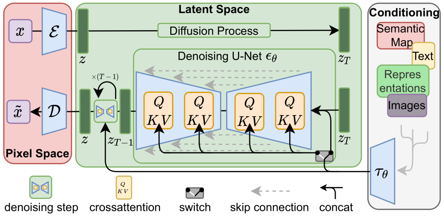
In summary, the T2I (i.e. text to image) [1,3] pipeline operates in the latent space, where the diffusion process begins with a random noise sample. Over T time steps, the process is conditioned on text encoding latent to iteratively denoise and generate an image that aligns with the input text.
Here’s how Inference works:
Input text is processed by a pre-trained text encoder, such as T5 or CLIP, encoding the semantic meaning as a fixed-length vector of embeddings.
Image generation starts with random noise in the latent (compressed) image space.
At each denoising step T, the model conditions the noise removal process on the text embedding.
Using cross-attention between image latent and text embedding, ensuring the generated closely matches the text prompt.
Noise is subtracted, producing a “clearer” latent representation of the image
The process repeats for many steps, gradually refining the latent noise + guided with text into a coherent latent image representation.
After the last Timestamp, the final latent representation is passed through the Autoencoder’s Decoder module, which constructs the vector back to a high-quality image.

Older versions of Stable Diffusion, such as v1, v1.5, and v2.1 base their model pipeline architecture on an LDM (i.e. Latent Diffusion Model). An LDM [10] consists of a VAE, U-Net, and a Text Encoder.
Within the LDM, the U-Net is used for denoising, which is well-suited for generating static images.
U-Nets in Latent Diffusion Models (LDMs)
The backbone of an LDM is a U-Net autoencoder with sparse connections providing a cross-attention mechanism. The U-Net predicts denoised image representation of noisy latents.
With it mainly being a CNN (i.e. Convolutional Neural Network) and while it can capture spatial information, it might struggle to maintain fine-grained spatial details, due to how Receptive Fields in Convolution Layers work.
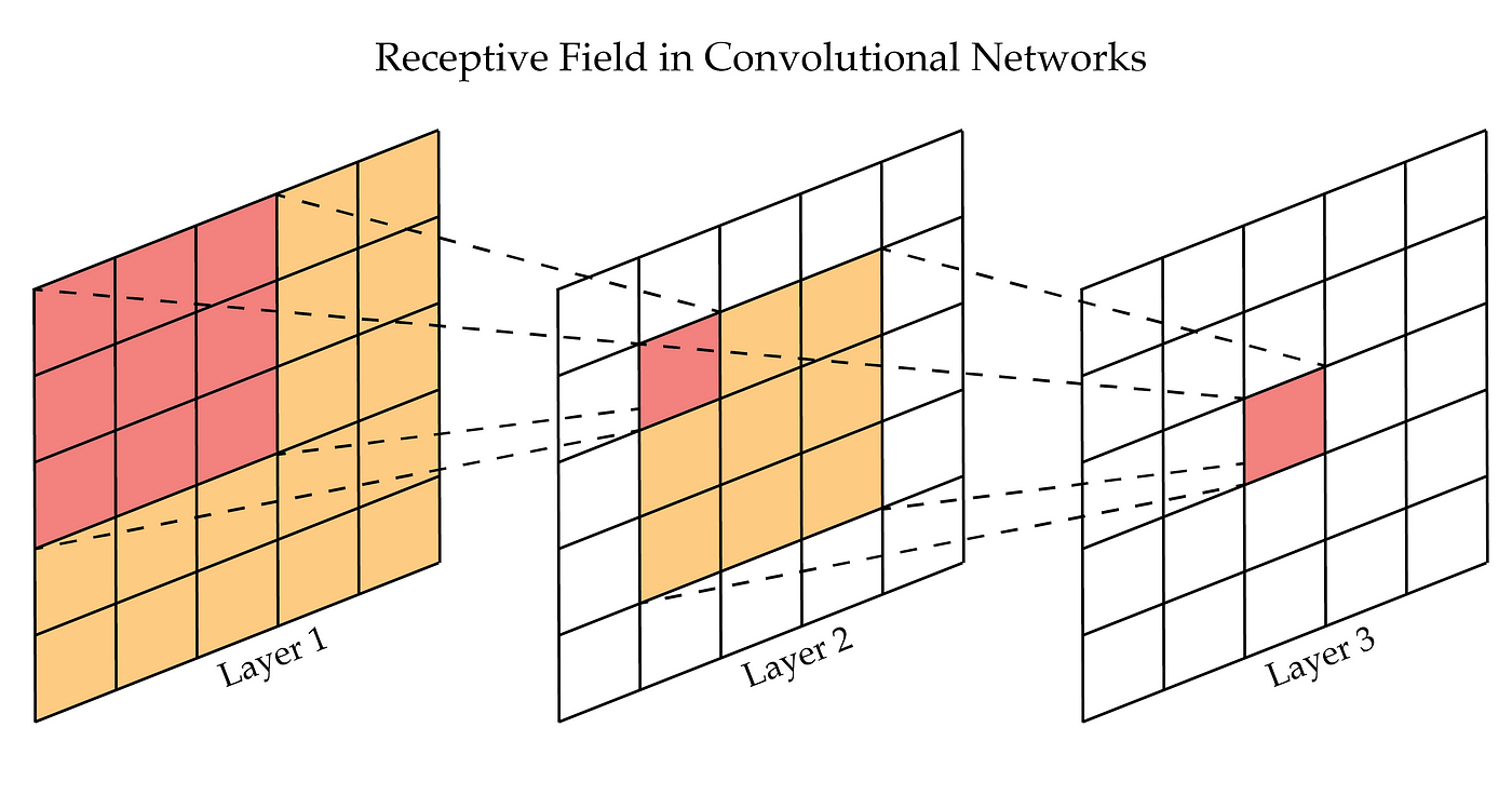
A Receptive Field is a region in the input space that a particular CNN's feature is affected by, and it’s local and finite.
We may imagine that a receptive field works as a pyramid.
If we take a CNN network architecture, and represent it in a top-down manner, with the input layer at the top and output layers at the bottom, imagine the receptive field “pyramid” as upside-down with its tip on the higher end of the network feature maps (i.e. deep layers), and the base at the lower end of the feature maps (i.e. first layers) of the network.
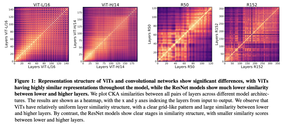
From the image above, we can see how continuous the feature similarity between low/high-level feature maps looks for ViT (i.e. Vision Transformer) and how fractured it is for Resnet-50/512 (i.e. CNN + Skip Connections).
That means - transformer models retain more structured spatial information than CNNs. Each image patch will have a link with all other image patches, similar to a “web”, because each element in the input interacts with all other elements, regardless of their distance. Each image patch embedding has a positional embedding, keeping information about the initial image structure.
In newer model iterations, such as Stable Diffusion 3 or FLUX models, the U-Net backend in the LDM model is replaced by a Diffusion Transformer.
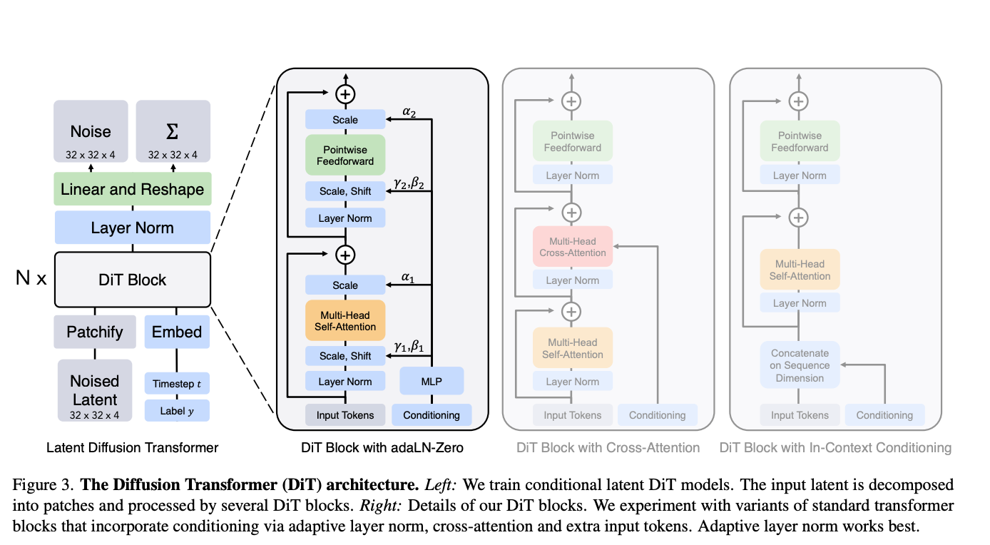
The Diffusion Transformer
The core idea of the Diffusion Transformer (DiT) is to use the Transformer as the backbone network for the diffusion model, instead of traditional convolutional neural networks (such as U-Net), to handle the latent representations of images.
Unlike CNNs, transformers can model long-range dependencies without the need for deep networks or large filters. Moreover, transformers are not translation invariant as they can capture the absolute position of features, thanks to positional encodings.
Two recent installments of T2I models which replaced the standard LDM & U-Net architecture with a Diffusion Transformer, are Stable Diffusion v3 [11] and Black Forrest Labs’s FLUX models.
Stability AI Stable Diffusion v3
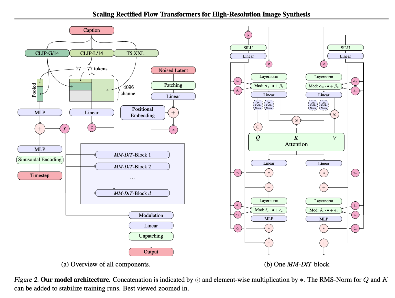
Using the text caption and a random noisy latent which is split into patches, the pair of caption embeddings and noisy latent patches which are positionally encoded pass through the DiT blocks for a series of diffusion timesteps. At the higher end of the model, the decoder unpacks the image latent into an actual image which the model returns.
FLUX (Black Forrest Labs)

Don't think there's a paper so had a quick look through their code. Might be useful for understanding current Diffusion architectures")
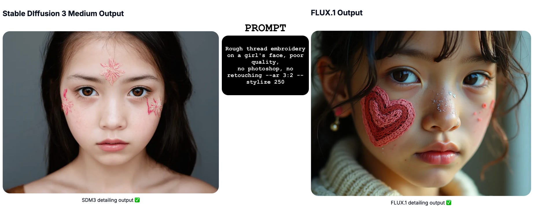
Stable Diffusion v3 vs FLUX
References
[1] O’Connor, R. (2022, May 12). Introduction to Diffusion Models for Machine Learning. News, Tutorials, AI Research.
[2] FLUX.1 vs Stable Diffusion 3. (2024). Aimlapi.com.
[3] Ho, J., Jain, A., & Abbeel, P. (2020). Denoising Diffusion Probabilistic Models.
[4] IBM. (2024, August 21). Diffusion models. Ibm.com.
[5] Lou, A. (2023). Reflected Diffusion Models | Aaron Lou. Aaronlou.com.
[6] Newhauser, M. (2023, July 13). The two models fueling generative AI products: Transformers and diffusion models. GPTech.
[7] black-forest-labs/FLUX.1-dev · Hugging Face. (2025). Huggingface.co.
[8] nrehiew (2024, August). FLUX-1 Unofficial architecture. X(Twitter).
[9] DALL·E 3. (2015). Openai.com.
[10] U-Net for Stable Diffusion. (2025). U-Net for Stable Diffusion.
[11] Esser, P., Kulal, S., Blattmann, A., Entezari, R., Müller, J., Saini, H., Levi, Y., Lorenz, D., Sauer, A., Boesel, F., Podell, D., Dockhorn, T., English, Z., Lacey, K., Goodwin, A., Marek, Y., & Rombach, R. (2024). Scaling Rectified Flow Transformers for High-Resolution Image Synthesis. ArXiv.org.
Text-to-Video Diffusion Models
Stepping up from T2I (i.e. text-to-image) models that generate a high-quality image closely related to the given prompt, T2V (i.e. text-to-video) models can create high-quality videos from a single text description. Below are a few takes on current SOTA models and their architecture proposals.
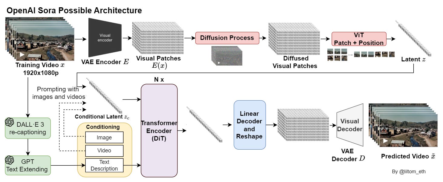
Sora, OpenAI

In Sora’s technical report [10], the authors specify that Sora is a diffusion transformer (DiT) [12], that was trained on latent compressed representations of videos.
What does that mean?
Well, to compress videos efficiently, they’ve trained a model to reduce the dimensionality of videos first, which takes a raw video as input and outputs a latent representation both temporally and spatially. At the same time, they also train a corresponding decoder model that maps generated latents back to pixel space.
Next, given a compressed input video, a sequence of spacetime patches is sampled, acting as transformer tokens. The diffusion process runs on these patches, denoising them into “clean” patches, guided by text modality, similar to how T2I (text-to-video) works for images.

While the complete Sora T2V pipeline architecture is proprietary, an open-world model architecture is being discussed on Twitter (X).
Make-a-Video, Facebook AI Research (FAIR)
Another photorealistic video generator works a little differently than OpenAI Sora in that it does not depend on text-video pairs. Still, instead, it scales on pre-trained T2I (i.e. text-to-image) diffusion models and subsequently utilizes unsupervised video to learn about motion.

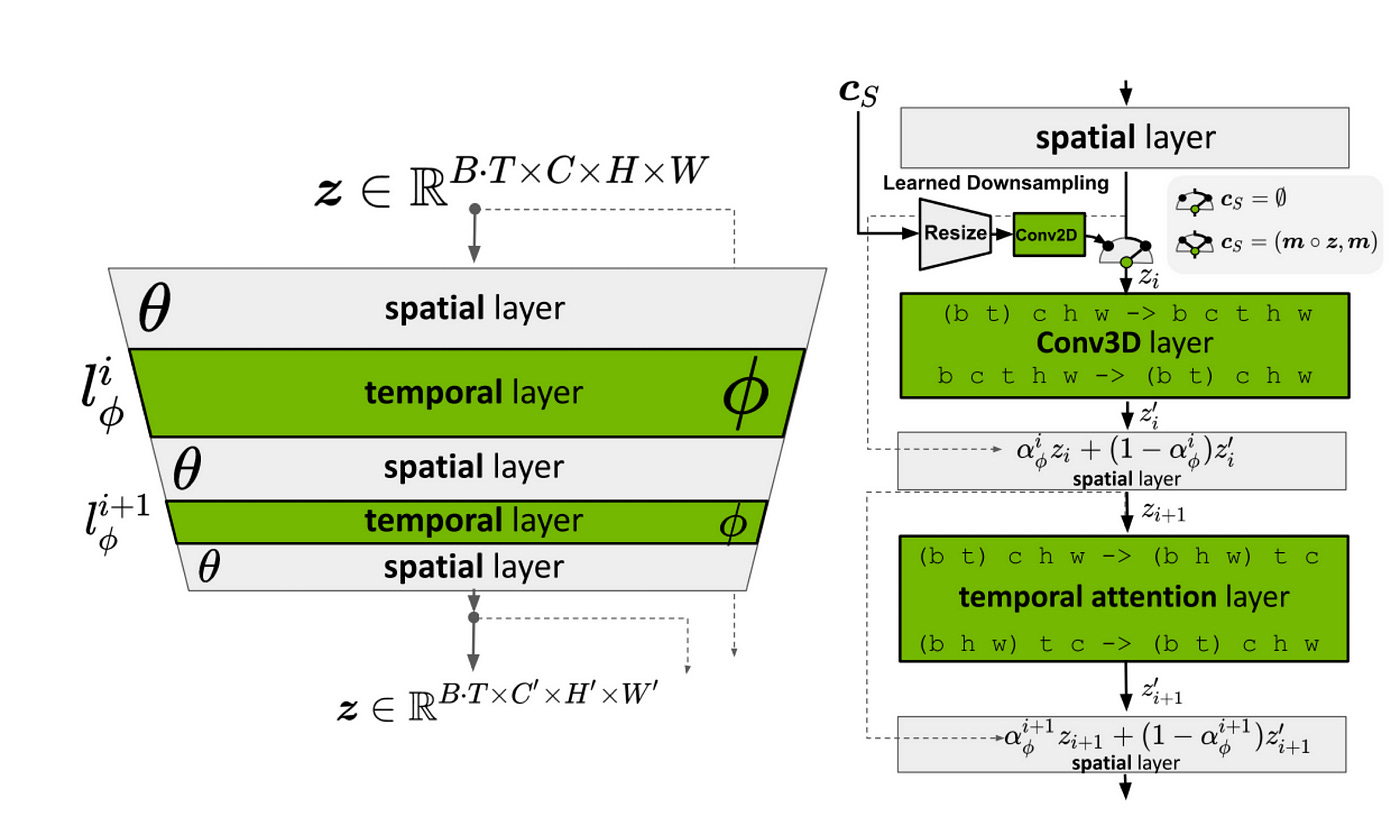
SVD, Image-to-Video Diffusion Models, NVIDIA
Stable Video Diffusion [8] (i.e. SVD) is a latent diffusion model trained to generate short video clips from image conditioning. This model was trained to generate 25 frames at a resolution of 576x1024 given a context frame of the same size.
Other notable T2V solutions are Runway ML Gen2 and Leonardo AI which offer T2V generation as a credit-based service SaaS.
References:
[1] Stability-AI/generative-models: Generative Models by Stability AI. (2023, July 27). GitHub.
[2] AI. (2023, November 21). Stability AI. Stability AI.
[3] Blattmann, A., Rombach, R., Ling, H., Dockhorn, T., Kim, S. W., Fidler, S., & Kreis, K. (2023). Align your Latents: High-Resolution Video Synthesis with Latent Diffusion Models. ArXiv.org.
[4] Gou, T. (2024, February 19). Techniques behind OpenAI Sora - Tom Gou - Medium. Medium.
[5] Blattmann, A., Dockhorn, T., Kulal, S., Mendelevitch, D., Kilian, M., Lorenz, D., Levi, Y., English, Z., Voleti, V., Letts, A., Jampani, V., & Rombach, R. (2023). Stable Video Diffusion: Scaling Latent Video Diffusion Models to Large Datasets. ArXiv.org.
[6] Singer, U., Polyak, A., Hayes, T., Xi, Jie, Y., Zhang, A., Hu, Q., Yang, H., Ashual, O., Gafni, O., Parikh, D., Gupta, S., Yaniv, & Ai, M. (n.d.). MAKE-A-VIDEO: TEXT-TO-VIDEO GENERATION WITHOUT TEXT-VIDEO DATA.
[7] Yang, Z., Teng, J., Zheng, W., Ding, M., Huang, S., Xu, J., Yang, Y., Hong, W., Zhang, X., Feng, G., Yin, D., Gu, X., Zhang, Y., Wang, W., Cheng, Y., Liu, T., Xu, B., Dong, Y., & Tang, J. (2024). CogVideoX: Text-to-Video Diffusion Models with An Expert Transformer. ArXiv.org.
[8] Jin, Y., Sun, Z., Li, N., Xu, K., Xu, K., Jiang, H., Zhuang, N., Huang, Q., Song, Y., Mu, Y., & Lin, Z. (2024). Pyramidal Flow Matching for Efficient Video Generative Modeling. ArXiv.org.
[9] hpcaitech/Open-Sora: Open-Sora: Democratizing Efficient Video Production for All. (2024, May 7). GitHub.
[10] Video generation models as world simulators. (2024). Openai.com.
[11] Raghu, M., Unterthiner, T., Kornblith, S., Zhang, C., & Dosovitskiy, A. (2021). Do Vision Transformers See Like Convolutional Neural Networks? ArXiv.org.
[12] Peebles, W., & Xie, S. (2022). Scalable Diffusion Models with Transformers. ArXiv.org.
Photorealistic 3D Scene Rendering (NeRF & Gaussian Splats)
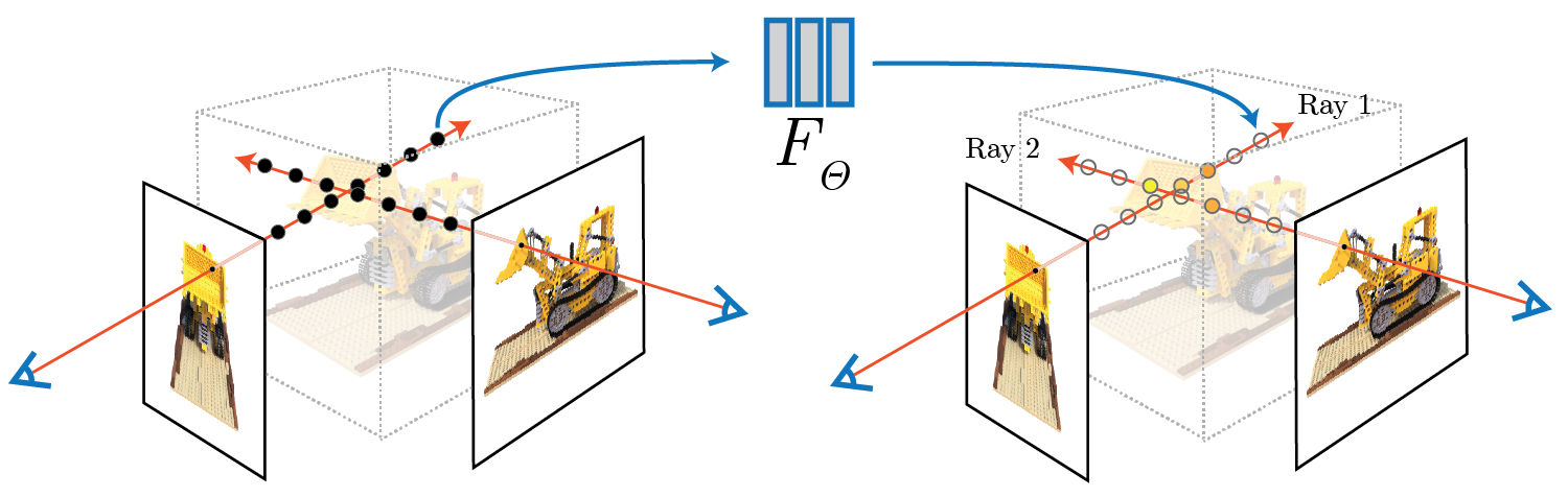
A neural radiance field (NeRF) is a neural network that can reconstruct complex 3D scenes from a partial set of 2D images, being able to learn the scene geometry, objects, and angles. Then it renders photorealistic 3D views from novel viewpoints, automatically generating synthetic data to fill in gaps.
The concept behind NeRFs is similar to how RayCasting shadows work in video game engines, where each ray of light produces a specific shadow intensity when it bounces off an object inside the scene.
With NeRFs, having a set of 2D images, for each pixel - it “casts” a ray across Z dimension, given that static images are XY, and at the position in XYZ where these pixel rays intersect, an intensity + color value is given to the 3D rendering. This relationship is learned by the model, which makes it able to generalize across multiple scene types.

Some of the most interesting NeRF applications in the real world is Google Maps and Street 3D renderings. In the video below (1:10min), in Google Maps, users can see the 3D rendering of any building, restaurant, or place and even do a virtual walkthrough in an AR (i.e. Augmented Reality) fashion.
References:
[1] NeRF: Neural Radiance Fields. (2020). Matthewtancik.com.
[2] Boesch, G. (2024, May 9). Neural Radiance Fields (NeRFs): A Technical Exploration - viso.ai. Viso.ai.
[3] Clayton, J. (2024, April 17). Moving Pictures: Transform Images Into 3D Scenes With NVIDIA Instant NeRF. NVIDIA Blog.
[4] Getting Started with NVIDIA Instant NeRFs | NVIDIA Technical Blog. (2022, May 12). NVIDIA Technical Blog.
Gaussian Splats
Rather than creating novel viewpoints using neural networks to estimate light radiance as NeRFs do, 3D Gaussian Splatting generates novel viewpoints by populating a 3D space with view-dependent “Gaussians.” These appear as fuzzy, 3D primitives with colors, densities, and positions adjusted to mimic light behavior.
Gaussian Splatting delivers photorealistic 3D reconstruction with generally improved visual quality and reduced generation times compared to NeRFs, positioning it as a state-of-the-art technique for 3D reconstruction.
We can think of Gaussian Splats as “blobs in space”. Instead of representing a 3D scene as polygonal meshes, voxels, or distance fields, it is represented as (millions of) particles:
Each particle (“a 3D Gaussian”) has a position, rotation, and a non-uniform scale in 3D space.
Each particle also has an opacity and color.
For rendering, the particles are rendered (“splatted”) as 2D Gaussians in screen space.
One downside of a rendered Gaussian Splatted scene is its size, as a single rendered image could take up to GBs of size on the disk.

References:
[1] aras-p/UnityGaussianSplatting: Toy Gaussian Splatting visualization in Unity. (2024, November 28). GitHub.
[2] 3D Gaussian Splatting: Performant 3D Scene Reconstruction at Scale | Amazon Web Services. (2024, August 27). Amazon Web Services.
[3] 3D Gaussian Splatting for Real-Time Radiance Field Rendering. (2023). Inria.fr.
Dude, this is CRAZY. Book quality. Amazing article 🚀